Introduction to R – Mathematics

One of the great things about mathematical and statistical programming is that makes gaining an intuition for how things work much easier because it lets the student actual perform operations they normally couldn’t. In this post we’ll use R and some elementary school level mathematics to demonstrate how numerical integration works.

 

Imagine a rocketship accelerating through space out of control. The only thing we know about the rocket is that the engine makes it accelerate at 5 m/s/s (five meters per second per second) and that it will run out of fuel after thirty seconds. To keep the solar system safe we want to know how fast it will end up going and how far it will travel the next minute.

There are so-called “analytical solutions” to this problem that were worked out by Isaac Newton a long time ago. Rather than use these equations of motion we’re going to retrace his steps. Let’s consider what we know:

• The rocket will reach its top speed after thirty seconds.
• It will travel some distance while accelerating.

First let’s make a vector that represents each moment spent accelerating. We’ll just call it time. Strictly speaking there are an infinite number of moments, of course, so we can only approximate a moment. I think a tenth of a second should be short enough. Using the seq() function makes this quite easy.

time <- seq(0,30,.1)

Now that we have a vector of moments in time we can evaluate the behavior of the rocket at each moment! Figuring out how fast its going is simple. Speed is acceleration multiplied by time. The tail() function shows us the last few values of the speed vector.

speed <- time*5
tail(speed)
147.5 148.0 148.5 149.0 149.5 150.0

There we see the final speed is 150 m/s. Of course we could have just multiplied 30 by 5 but we’re going to need that vector of speeds for the next part.

How far does the rocket travel? After the rocket stops accelerating that’s easy to figure out. Distance is speed multiplied by time, if you go 60 miles per hour for an hour you’ll travel 60 miles. There will be another thirty seconds left once the rocket stops accelerating.

150*30
4500

But how to figure out the distance traveled while accelerating when the speed is changing all the time? Since the we know the speed of the rocket at each moment and we know that each “moment” is a tenth of a second we can use exactly the same math there as well, we just have to go moment by moment.

distance <- speed*.1

Now what? We have a vector of distances but we want a single number, the total distance. The sum() function quickly adds up all of the values for us.

sum(distance)
2257.5

Finally we can just take the distance travel while accelerating and add it to the distance traveled afterward.

2257.5+4500
6757.5

Finally let’s use R to visualize the movement of the rocket. We’ll make the distance that it spends traveling at a constant speed into a vector as well and combine that with the ‘distance’ vector. The rep() function will repeat 15 meters (the distance traveled every tenth of a second) the appropriate number of times.

distance2 <- rep(15,300)
combined <- c(distance,distance2)

The cumsum() function calculates the cumulative sum of the distances. We’ll make a new time vector so that the graph looks nicer when we plot it.

total <- cumsum(combined)
time <- seq(0,60,.1)
plot(x=time,y=total)

That’s exactly what it should look like. First we see a curve as it accelerates then we see a straight line when it runs out of fuel and continues traveling at 150m/s for another thirty seconds.

As an exercise for the reader take the code used in this post and see which parts you can combine to do the calculations in fewer lines.

In the next post we will jump into the deep end to take a look at creating a custom function in R.

Introduction to R – Dataframes

The third, and most important, kind of R object we will study is called a dataframe, which is how R typically stores statistical data. Although you can make them on your own with the data.frame() function a lot of them come built in or can be downloaded as needed.

To start we’ll make our own dataframe using the results of the 2014 Boston Marathon Wheelchair Division. The data is made up of several vectors. The placement of the racer, their sex, the time (in minutes) they took to finish, and the country they raced for. Feel free to copy and paste these rather than type them out by hand.

Place <- c(1:5,1:5)
Sex <- c(rep("Male",5),rep("Female",5))
Time <- c(80.60,81.23,81.23,84.65,84.70,95.10,97.40,98.55,99.65,101.70)
Country <- c("RSA","JPN","JPN","SUI","ESP","USA","JPN","USA","SUI","GBR")

Now we use the data.frame() function to combine them.

boston <- data.frame(Place,Sex,Time,Country)
boston
   Place    Sex   Time Country
1      1   Male  80.60     RSA
2      2   Male  81.23     JPN
3      3   Male  81.23     JPN
4      4   Male  84.65     SUI
5      5   Male  84.70     ESP
6      1 Female  95.10     USA
7      2 Female  97.40     JPN
8      3 Female  98.55     USA
9      4 Female  99.65     SUI
10     5 Female 101.70     GBR

Short and easy to understand. Each line represents a single person. Line 8 is the third place woman she was an American who took 98.55 minutes to complete the race. You may notice that a dataframe is somewhat like a matrix. The largest difference is in how R treats them, a number of functions work especially well with dataframes. Since we have this convenient dataframe to work with let’s take the opportunity to learn about structure with the str() function.

str(boston)
'data.frame':   10 obs. of  4 variables:
 $ Place  : int  1 2 3 4 5 1 2 3 4 5
 $ Sex    : Factor w/ 2 levels "Female","Male": 2 2 2 2 2 1 1 1 1 1
 $ Time   : num  80.6 81.2 81.2 84.7 84.7 ...
 $ Country: Factor w/ 6 levels "ESP","GBR","JPN",..: 4 3 3 5 1 6 3 6 5 2

Race results are good because they include many different kinds of data and this gives us a chance to see how R treats them. We’ll talk about levels of measurement in a later post but for now notice the information that str() gives you about the data.

There are “10 obs. of 4 variables” which means the dataframe is ten lines long and has four pieces of information (Place, Sex, Time, and Country). Next it tells you about each variable. The Place variable is made of integers, whole numbers only. The Sex variable is a “Factor w/ 2 levels” which means the information does not have a numerical form and there are two options. The Time variable is a numeric which means it can hold any numerical value, including decimals. The Country variable is a “Factor w/ 6 levels” which means that, like Sex, it doesn’t have numerical form and there are six options.

Since the boston data is extremely small you could have figured all of this out by yourself but in practice dataframe can be thousands of lines long and have many variables. With the str() function you can get a simple explanation of all of them.

The subsetting notation we saw before with vectors and matrices also works with dataframes. For example let’s look at row seven.

boston[7,]
  Place    Sex Time Country
7     2 Female 97.4     JPN

All of the columns in dataframes are variables with names and names are easier to remember than the column numbers so R allows you to extract a variable by using its name. To extract the variables you can use $ notation as well as the [ ] notation. These commands are all equivalent.

boston$Time
boston[,3]
boston[,"Time"]

Now that we have a dataframe to play with we can look at more complex subsetting commands that are frequently useful. Let’s look at a few of them. See if you can follow along, we’re just combining commands we’ve seen before, essentially making subsets of subsets.

Only the Japanese racers:

boston[boston$Country=="JPN",]
  Place    Sex  Time Country
2     2   Male 81.23     JPN
3     3   Male 81.23     JPN
7     2 Female 97.40     JPN

Only the woman in first place:

boston[boston$Sex=="Female" & boston$Place==1,]
  Place    Sex Time Country
6     1 Female 95.1     USA

It’s also possible to apply functions to subsets. For example let’s look at the average of the times and then average for each of men and women by using the mean() function on different pieces of the dataframe.

mean(boston$Time)
90.481
mean(boston$Time[boston$Sex=="Male"])
82.482
mean(boston$Time[boston$Sex=="Female"])
98.48

The boston data is extremely small and simple. You could probably understand everything you want to know about it just by looking at the whole thing. In practice you’ll want to use R with data that is significantly larger and more complicated. The Old Faithful data is one of the most frequently analyzed data sets in all of statistics. It comes built into R as the faithful dataframe which you can call up any time you want.

Because it is much larger than boston we should start with the str() function in order to understand it.

str(faithful)
'data.frame':   272 obs. of  2 variables:
 $ eruptions: num  3.6 1.8 3.33 2.28 4.53 ...
 $ waiting  : num  79 54 74 62 85 55 88 85 51 85 ...

That’s actually smaller than the structure of the boston data because there are only two variables but take a look at that first line. Yep, faithful has 272 rows! That’s much too large for us to try and understand just by looking at the whole dataframe. Read the descriptions of that eruptions variable and the waiting variable to see what they tell you.

Since faithful is built into R you can get detailed information from the internet by using the help function.

?faithful

That webpage tells us that the eruptions variable is the length of the eruption in minutes and the waiting variable is the delay between that eruption and the next. The task of a data scientist is to transform data into information, so that we can eventually gain knowledge. There are countless ways of getting information out of the data. One of the most popular is to calculate summary statistics. The summary() function computes several popular ones, all of which can be calculated individual if you’d prefer.

summary(faithful)
   eruptions        waiting
 Min.   :1.600   Min.   :43.0
 1st Qu.:2.163   1st Qu.:58.0
 Median :4.000   Median :76.0
 Mean   :3.488   Mean   :70.9
 3rd Qu.:4.454   3rd Qu.:82.0
 Max.   :5.100   Max.   :96.0

The min() and max() are the smallest and largest values. The mean() is the average value. The median() is the central value. The 1st and 3rd quartiles mark the bottom 25% and top 25% of the data, exactly half of the data falls between those values.

We can see here that old faithful isn’t quite as faithful as you may have been lead to believe. The eruptions range from 1.6 to 5.1 minutes in duration and occur between 43 and 96 minutes apart. Even if we look at the quartiles, to ignore outliers, there is a significant degree of variability.

There is a better way. Watch this:

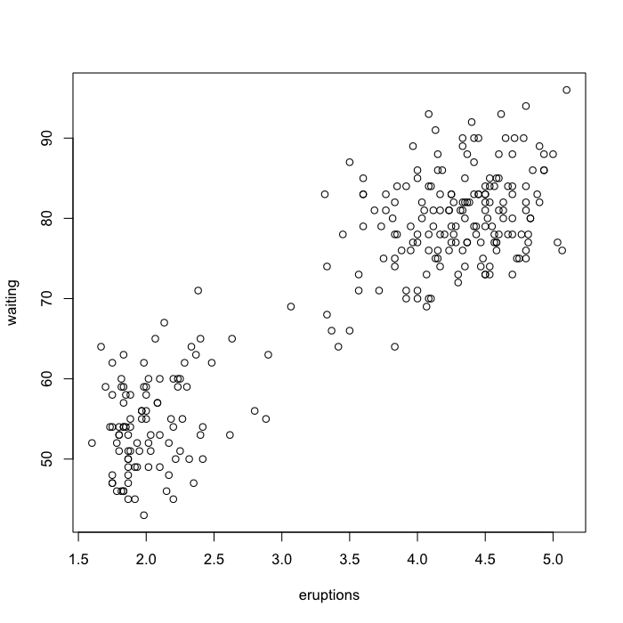
plot(faithful)

The ease with which basic graphics can be made is one of the best things about R. More complex visualizations are better done with one of the many graphics packages available but base R graphics can efficiently do a lot of work. Looking at the plot we see that there are basically two kinds of eruptions, long ones that are followed by a long delay and short ones that are followed by a short delay.

The additional drawing functions let us quickly add things to the graphics we make. Let’s draw a line dividing the two groups. Crudely we might draw it at the mean of the eruption duration. While the scatterplot is open use the abline() function to draw a straight vertical line.

abline(v=mean(faithful$eruptions))

Finally lets look at a smaller but more complex dataframe called mtcars. It is only 32 lines long but each type of car was measured for 11 variables. You’ve made use of the srt() and plot() functions before so try theme with mtcars on your own. See what conclusions you can draw then using the ? function to learn more about it.

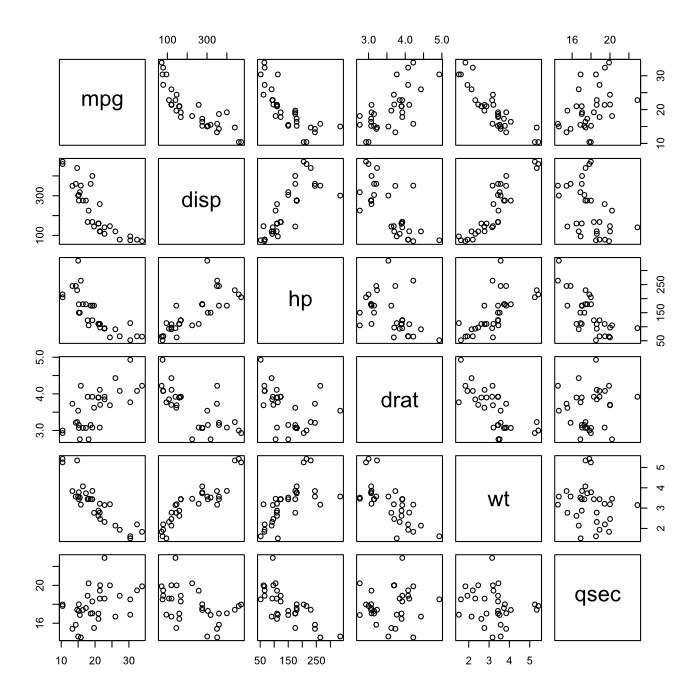
When you tried the plot() function you probably got a huge grid of scatterplots. This scatterplot matrix can be intimidating but it really isn’t that different from a normal scatterplot. Let’s use the subsetting notation to look at just a few of the variables.

plot(mtcars[,c("mpg","disp","hp","drat","wt","qsec")])

Take a second to examine this line of code, you should already be familiar with each part of it. We use the plot() function on a subset of mtcars that we define with a vector made up of strings, thanks to the c() function we learned about earlier.

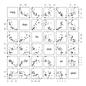
To read a plot matrix find the place where the two variables you’re interested in intersect. For example immediately below the mpg (miles per gallon) cell is the scatterplot showing its relationship to the disp (displacement or volume) of the car. It looks to me like as the size of the car increases mileage decreases. The same relationship looks to be true of mpg and hp (horsepower) while the opposite is true of wt (weight) an disp.

In the next post we’ll take a look at solving and visualizing a simple problem in R as a way to practice working with data.

Introduction to R – Vectors

In the last post we discussed how to do basic math with R and introduced the concept of objects. As important as scalar objects are, they are only the most basic kind of object in R. In this post we will talk about vectors.

The fundamental building block of R is called a vector and clever use of vectors is the language’s greatest strength. Fortunately a vector isn’t an harder to understand than a scalar is. A vector consists of several elements in a particular order, nothing more and nothing less. Each element of a vector is a number or a string. Since order matters a vector that contains the sequence 1, 2, 3 is different from one that contains 3, 2, 1.

To make a vector we use a function called c(), which is short for “concatenate”, which is long for “put in order”. An object can be a vector exactly like it can be a number or word. The same assign function we used for making objects before is used again. In fact we will keep using the assign function no matter how deep we get into R.

d <- c(1,2,3,4,5)
e <- c(2,2,3,8,1)

d
1 2 3 4 5

e
2 2 3 8 1

aVectorOfStrings <- c("Hello","World")
aVectorOfStrings
"Hello" "World"

Doing math with these vectors uses the familiar operations you already know.

d+5
6 7 8 9 10

As you can see five has been added to each element of the vector. Rather than write a loop the way other programming languages would ask you to do R already knows exactly what to do with a vector from the very beginning. When we do math with vectors rather than writing loops of code it is called vectorization and R can do it with blazing speed. Need to know the natural logarithm of every number from 1 to 1000000 for some reason? A fraction of a second.

Try using ‘d’ and ‘e’ with some operations that interest you before we continue.

What are the elements of ‘d’ right now after we’ve added to it and done all the things you wanted to?

d
1 2 3 4 5

For some reasons ‘d’ hasn’t changed at all! Why? Because we didn’t use the assign function on it. R won’t overwrite objects unless we actually tell it to. Let’s try again.

d <- d+5
d
6 7 8 9 10

What about when we use two vectors rather than one? Can you multiply ‘d’ by ‘e’? What would that even mean? It never hurts to experiment when learning so let’s try it.

d*e
12 14 24 72 10

That’s a new vector with five elements to it, the same length as both ‘d’ and ‘e’. Notice that the values are made by combining the two vectors in order. 12 is 6*2. 14 is 7*2. 24 is 8*3. And so on and so on. The same is true of any operation you like.

We should also start getting in the habit of assigning a name to everything we do. It’s very useful to store things as you go since you never know when you might want them again. On your own use the assign function to make an object called ‘de’ that contains d*e.

It’s often important to be able to get information out of vectors and other objects, perhaps we just want to know the value of a particular element in a vector. The subsettting notation is how we do this. Using brackets we just write the position we’d like to get after the name of the vector.

The second element of ‘d’ and the fifth element of ‘e’.

d[2]
7
e[5]
1

Remember that if you can do something with a scalar, a single number, R will often let you do it with a vector as well. If you put a vector into the brackets you can extract several values from an object all at once. How about the 1^st, 3^rd, and 5^th elements of de?

de[c(1,3,5)]
12 24 10

Since everything in R can be made into an object you might already have guessed that you can use the assign function to save subsets. Thanks to this efficient notation taking a portion of an object to work with separate from the whole, which is quite common, is quick and simple. Try making a few objects that are subsets of other objects on your own.

Since vectors are so important to R you should take some time to play around with them. Take some time to play around with vectors and get comfortable using them. More than anything else they are the core of understanding how to think about R.

The nearest relative of vectors is called a matrix. Where a vector is many values in a particular order a matrix is many values each in a particular position on a grid. A matrix can be made by using the matrix() function and providing a vector with all the values to go in the matrix. This is how we make a two by three matrix.

First we make a vector.

s <- c(1,2,3,4,5,6)

Then we define the matrix. First we tell it the data to use, the vector we just made, and then the number of row and the number of columns.

m <- matrix(s,2,3)
     [,1] [,2] [,3]
[1,]    1    3    5
[2,]    2    4    6

Notice that it’s simply a grid of numbers in the same way that a vector was simply a line of numbers. We use the same subsetting notation to get values out of the matrix but now we specify the rows and columns. The row is written first then the column.

m[1,2]
3

If you leave out the column number you get the whole row. If you leave out the row number you get the whole column.

m[1,]
1 3 5

m[,1]
1 2

Matrices are used much less often than vectors but its is still useful to be familiar with them since they’re a slightly more complex structure than a vector. We will also be seeing the same subsetting notation we used here later for other kinds of objects.

Try making a matrix of your own and see how it reacts to mathematical operations, it’s much the same as using a vector. Don’t be afraid to copy the code I have written here and modify it, that’s one of the best ways to learn.

Before we move on to data objects let’s look at one special way to make a vector and one special way to work with vectors. Its common to want a sequence of numbers in a vector and writing that out by hand is exhausting, the designers didn’t want us to get carpal tunnel syndrome. As a result R provides the seq() function to speed the creation of long sequences.

long <- seq(from=1,to=100,by=1)

I won’t print the contents of ‘long’ here because its has one hundred elements but notice that the seq() function takes arguments, in this case “from”, “to”, and “by”. We have told R to make a sequence that starts at 1 and ends at 100 counting by 1 each time. Which just means it makes a vector that goes 1, 2, 3, 4, 5 and so on until you reach 100. Sequences that go by 1 are so common they even have special notation. The following command is identical to the one we just used.

long <- 1:100

Try making a matrix that will hold ‘long’, it needs ten columns and ten rows. Try doing some mathematical operations with ‘long’ as well. You’ll soon see that using a large vector isn’t really an different from working with a shorter one.

Finally let’s talk about collapsing vectors and matrices. Just like writing out a long vector is impractical so is adding up all of the values in it. There are analytical solutions to some of these problems but a vector might contain a thousand completely random numbers! The sum() function, short for summation, does this for us by automatically adding up all of the elements of a vector.

sum(long)
5050

The prod() function, short for product, does the same thing with multiplication.

Now that you’ve had an introduction to the basic objects that are a part of R we look at data objects in the next post, before applying what we’ve learned to simple problem solving.

The Absolute Introduction to R

Today I begin my series “The Absolute Introduction to R” based on the premise that you know nothing about programming and only a little bit about statistics. The benefit of R over statistical programs is that it is infinitely flexible. If you can describe what you want to do then you can write a program to do it. R is also extremely compact. Even elaborate analysis can be done in just a few lines of code because R has been designed with statistics in mind.

R is an open source programming language used in statistics and data science. Installing R is as simple as installing any other program on a computer. It can be downloaded in a few minutes from CRAN.

http://cran.r-project.org/bin/windows/base/

Once you have installed R open it up and we’ll get started.

The R console should look something like this. To input commands or build programs type directly into the console then press enter to execute the command. Alternatively go to File -> New Script to open up a script. You can write several lines at once in a script and then execute all of them by highlighting them and pressing Ctrl+R. Try both methods as we go.

The most basic use of R is as a simple calculator. Doing elementary math is as simple as typing out the equation you want to perform.

First let’s look at addition and subtraction:

3+4
7
3-4
-1

Now multiplication and division:

3*4
12
3/4
0.75

The bracketed 1 at the beginning of each line is simply to tell you that it is the first output of the operation. Later we will see operations that produce many outputs and the bracketed numbers will help you keep track of them but for now we will have only a single line.

For the most part this tutorial will use only addition and multiplication. What we will do is use R to transform those very simple operations into much more powerful tools. If you wish take some time to play around with using R as a calculator. You can do any operation (math problem) you can think of.

A few more complex operations just for the sake of completeness. We won’t be using any of these but its nice to see that these, perhaps mysterious, operations are no more difficult to write out than the elementary ones. Being able to quickly call up these operations ultimately makes understanding them vastly simpler.

Exponentiation:

10^3
1000

The natural and common logarithms:

log(4)
1.386294
log10(1000)
3

Roots:

sqrt(3)
1.732051
3^(1/4)
1.316074

Factorials:

factorial(4)
24

When you’re ready to continue go on to the next part and we’ll examine the next step in using R. You can clean up the console with the command Ctrl+L rather than leave it cluttered with equations. Doing math this way can be cumbersome and R has myriad more complex operations built in that we can use. We’ll seem them later but first let’s take a look at the building blocks of programs.

Like many programming languages objects are a core part of R. An object is just what it sounds like a “thing” in R that you can do things to. Numbers are objects. Words are objects. Datasets are objects. We will even get to define our own objects as we go. Getting access to an object is as simple as typing its name into the console. The famous number pi, for instance, comes built in to R.

pi
3.141593

We frequently need to define our own objects, though. In R this is done with the assign function <-. Let's make an object that contains the number 7.

a <- 7
a
7

Simple as that from now until you close the program R will treat the object 'a' exactly as if it were the number seven. This might not sound useful now but pretty soon well see how objects can save us a huge amount of space and time. Simple objects like this are not a passing introductory example, though, they remain critical even is the mot complex programs you can devise.

These objects are called a numeric because they both contain a number. This is why we can use them in math problems.

a+2
9
pi/2
1.570796

Objects that contain text rather than numbers are known as strings. Here's an example of an object that contains the phrase Hello World.

somewords <- “Hello World”
somewords
“Hello World”

Notice that when we make this object we have to put Hello World in quotes so that R knows we're giving it some text. If we didn't include the quotes R would think that Hello and World were objects we wanted to reference, neither of which exists yet! We won't make much use a strings in this introduction because they can't be used to do mathematics but they're very helpful when making graphics.

R remembers objects you make…

a
7
somewords
“Hello World”

…but it is very specific about how you write them.

Error: object 'A' not found
SomeWords
Error: object 'SomeWords' not found

A name has to be the same in every way, no changing capitalization or adding characters or symbols to it. Object names also cannot include any spaces. All of these names have absolutely no relation to each other as far as R is concerned:

mydata
MyData
my.data
MYDATA

The ability to assign objects a name is very powerful, we can define an object that will hold anything else in R that you can create The mighty outputs of generalized linear models and Monte Carlo Markov Chains can be held within the confines of a single letter!

An object that contains only a single value is called a scalar. So far all of these objects we've made have been scalars. They hold a single number or a single string like a variable in an algebra problem. Play around with scalars for a while. You'll soon see that numeric scalars (fancy language isn’t it?) can be used to do any familiar mathematical operations from addition to logarithms.

In the next post we will look at vectors, a very important kind of simple object, and then we will move on to data objects.