The Circle – Sine and Cosine

In high school people are usually taught the three trigonometric functions, which is odd because there are a lot more than that, nine that see regular use. They can be thought of as three pairs of three starting with the sine, cosine, and tangent. It takes a bit of work to draw each of these functions so the code is presented at the end of the post rather than with each graphic.

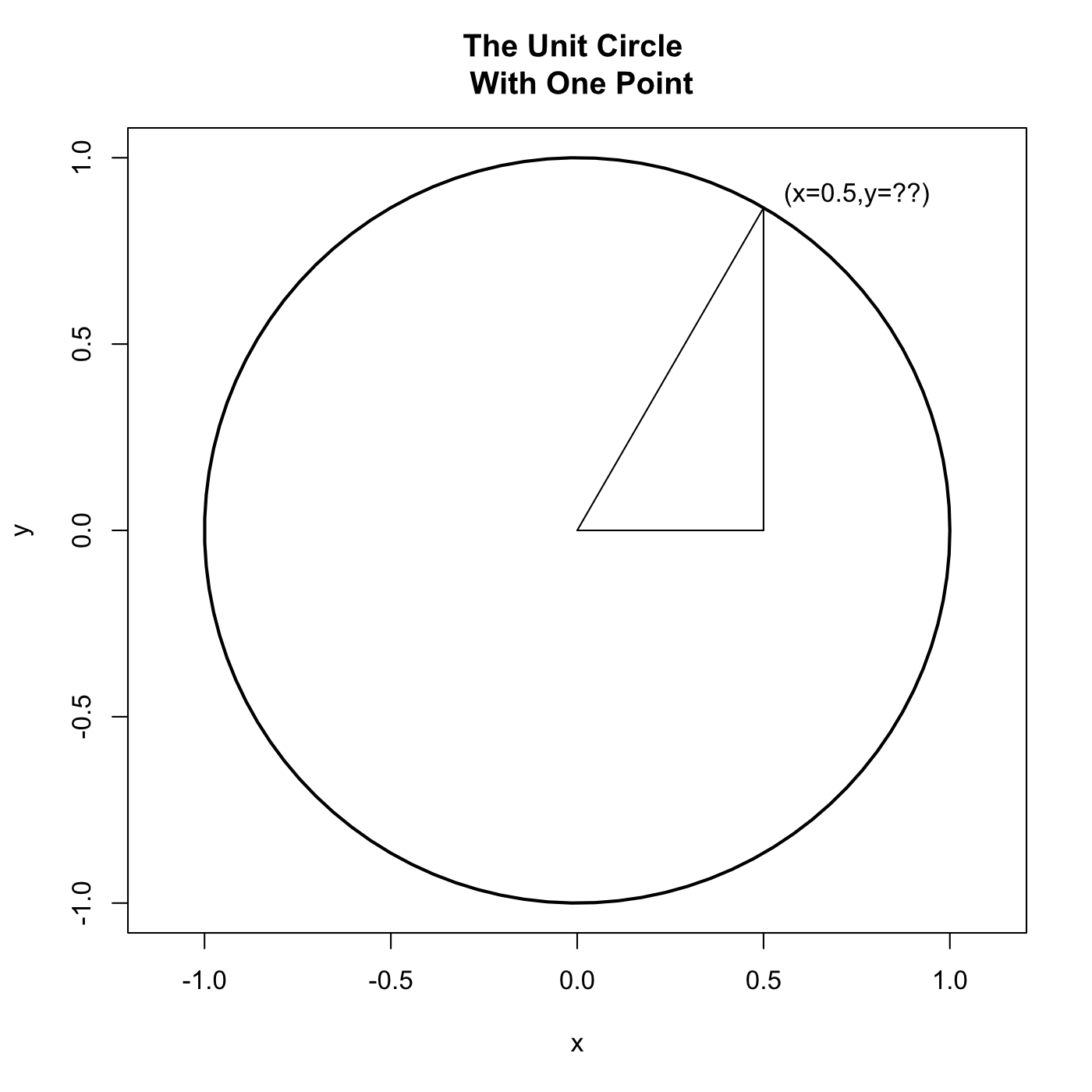
Let’s draw a circle and use it to construct the values of the functions. All of them correspond to a characteristic of a triangle draw on the circle. Let’s start with the sine and cosine because they have the most natural representations.

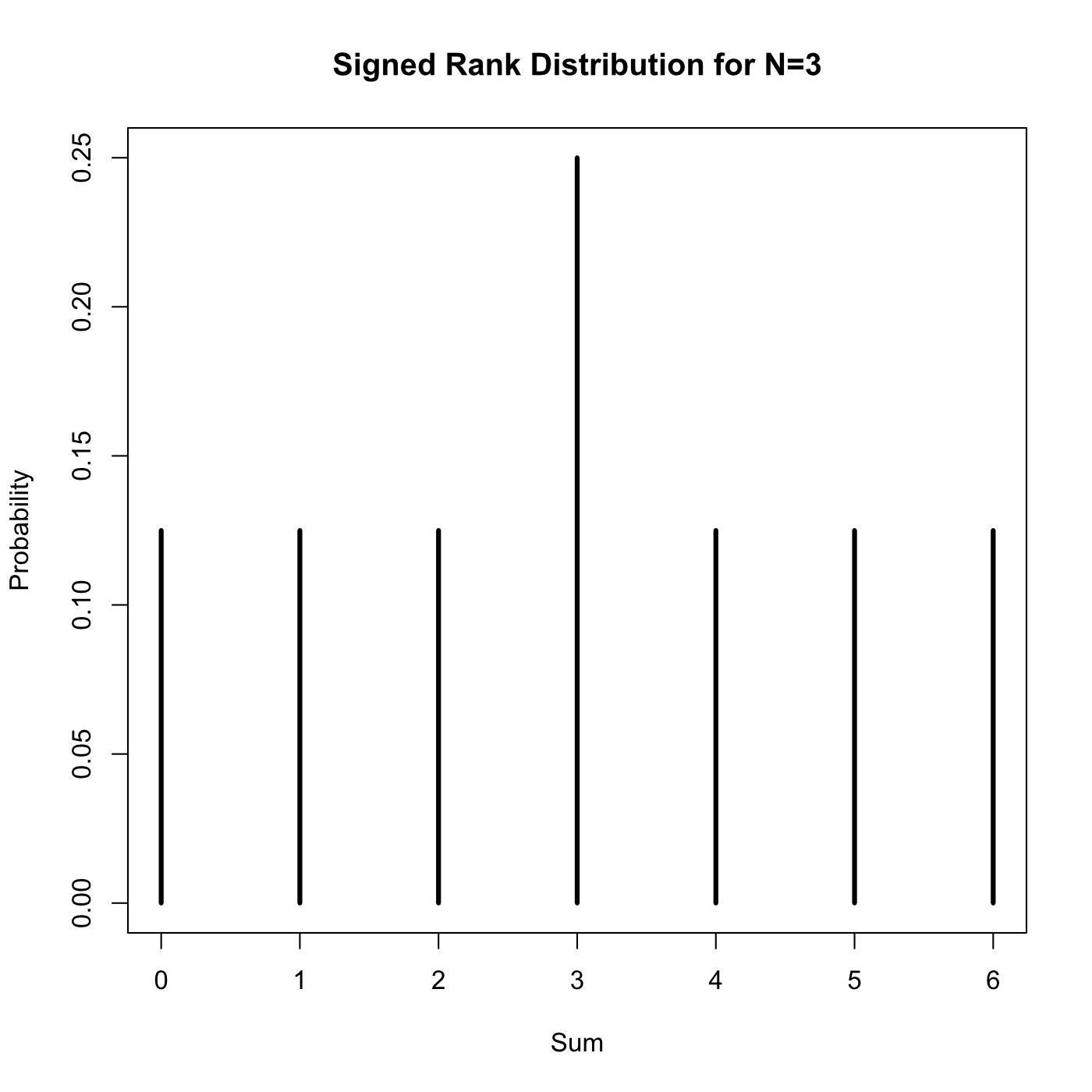
Here are the sine and cosine:

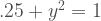
They have the length of those two colored lines respectively. The length of those lines is completely determined by the length of the radius and the angle of theta. In this case the angle is 1 radian and the radius of the unit circle is exactly equal to 1 so we can use R to find that . . .

sin(1)
[1] 0.841471
cos(1)
[1] 0.5403023

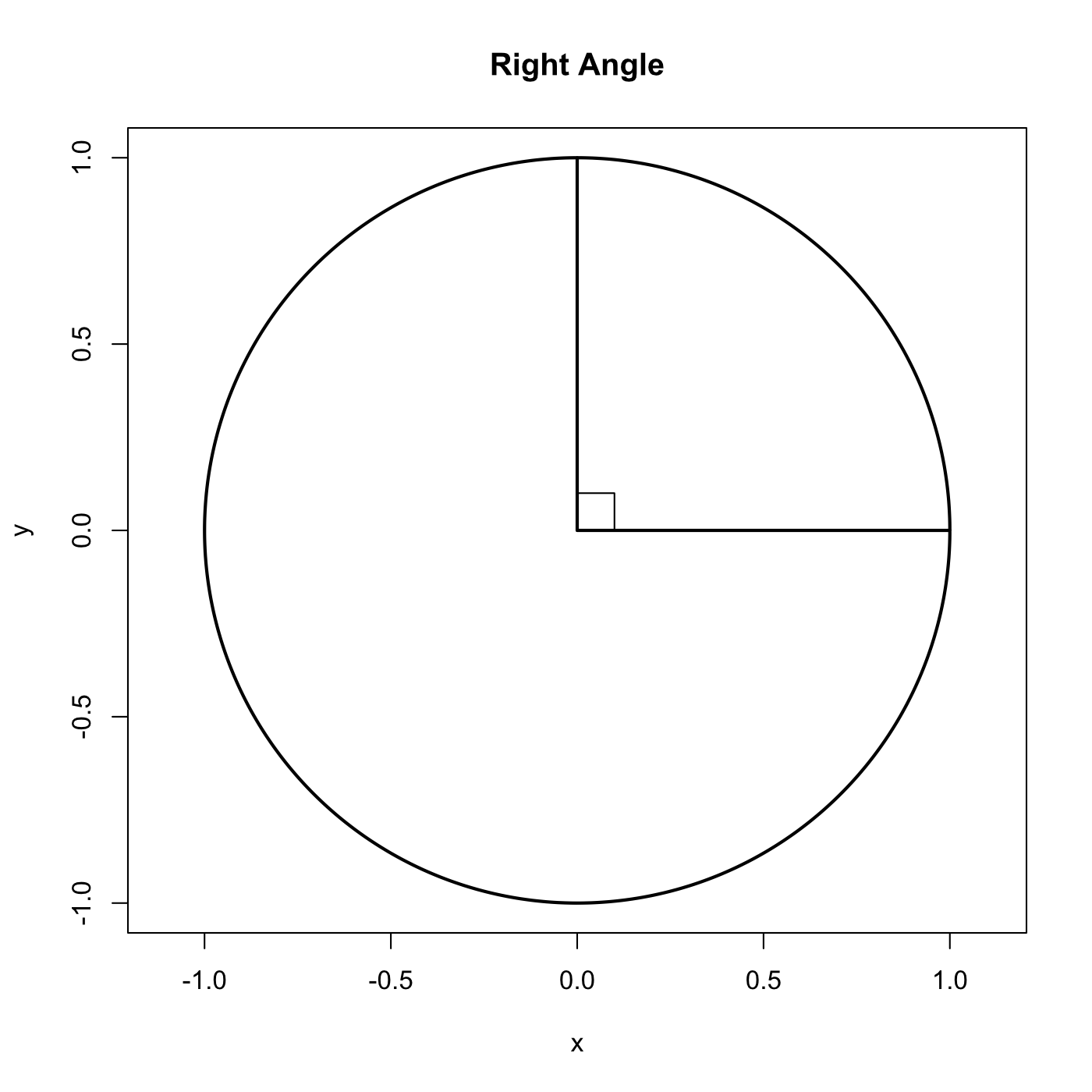
In other words the sine of theta gives us the y-coordinate of a point on the unit circle and the cosine of theta gives us the x-coordinate of that same point. Just by looking at the image we can intuit certain properties of the two functions. Both of them vary between -1 and 1, the bounds of the circle, and they’re offset by exactly 90 degrees (π/2 radians) which means that the sine of π is the same the cosine of π/2.

If we plot how the vales of the sin and cosine change with in inputs we get a pair of waves.

x <- seq(-5,5,.1)
y1 <- sin(x)
y2 <- cos(x)

plot(y1~x,
	main = 'Sine and Cosine Waves',
	lwd = 3, col = 'blue', type = 'l',
	ylim = c(-2,2))
lines(y2~x, lwd = 3, col = 'darkorchid')

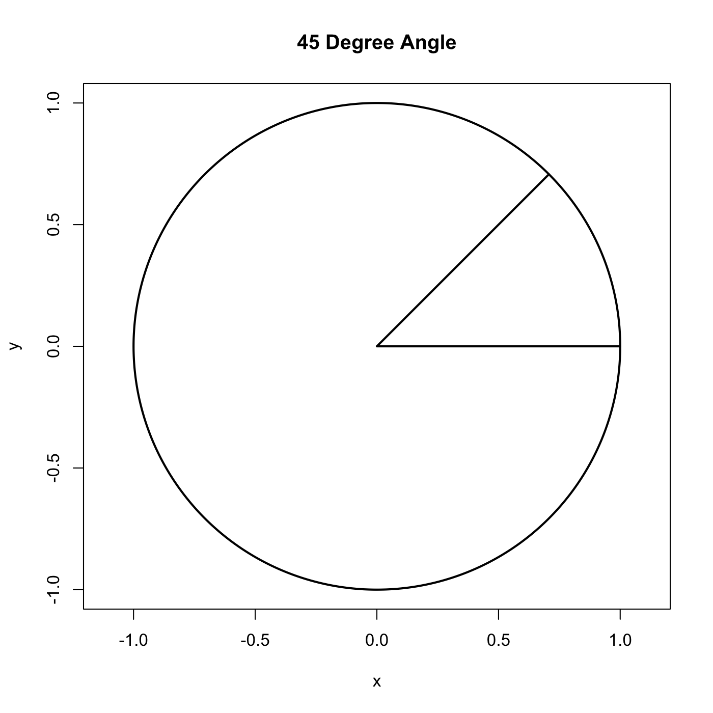
These are are the shape that you see on oscilloscopes in old science fiction movies (or at work if you often measure voltages). You can see that there are points where the two curves cross at all of the multiples of π/4 (a 45 degree angle).

Notice that the three lines (radius, sine, and cosine) together describe a right triangle. Because of this the trigonometric functions can be used to solve triangles and then to solve much more complex structures because we can build them out of triangles. If we vary the radius of the circle the length of the other lines scale proportionally. In fact this is true for all of the trigonometric functions. As a result we can simply a lot of things by working on the unit circle and then scaling appropriately when we’re done.

Let’s use this fact to derive an important fact about the sine and cosine.

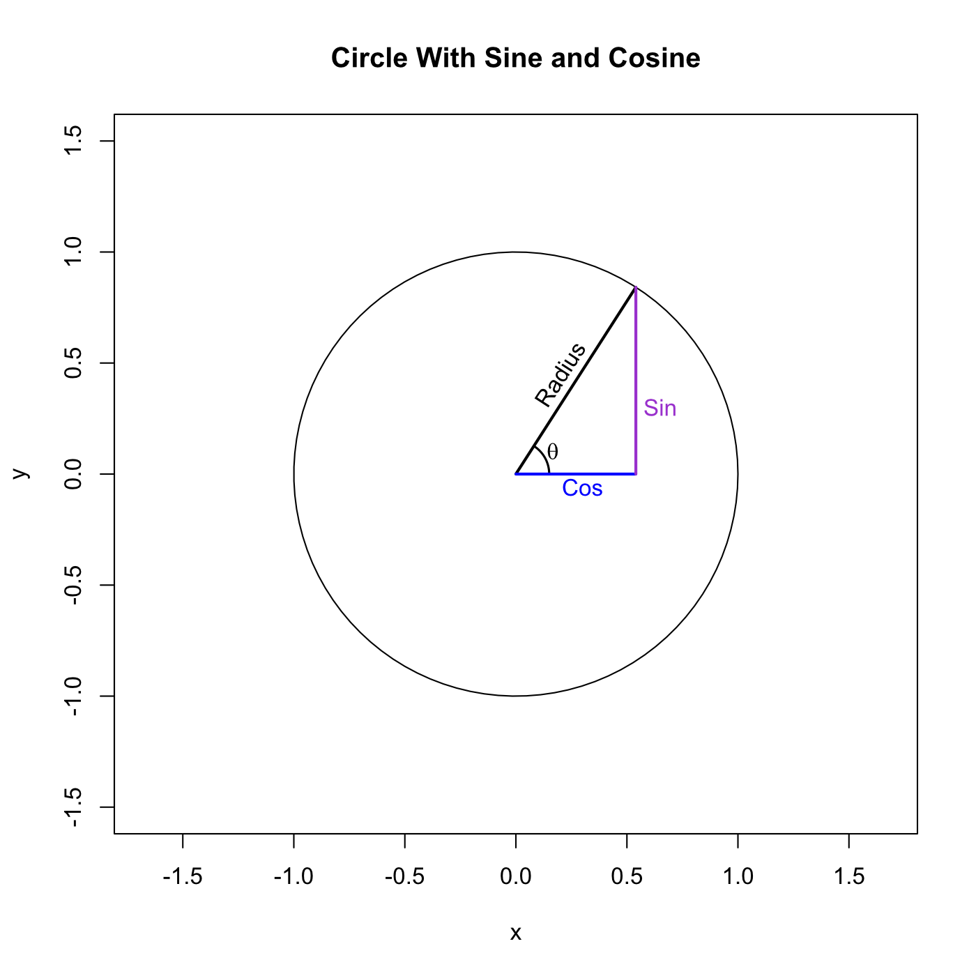
Using the sine, cosine, and tangent it is possible to fully describe a right triangle with just a few pieces of information. Consider a simple right triangle on a circle with angles of A = 1, B = 0.57, the third angle is π/2 since its a right angle.

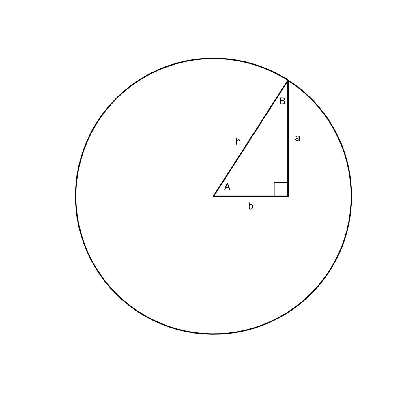
The sine of angle A is 0.84 so we know that side a has a length of 0.84r and the cosine of A is 0.54 so we know that the length of side b is 0.54r, where r is the length of the hypotenuse (or the radius). This follows quite obviously from the definition of sine and cosine and the properties we’ve discussed. The only piece of information we don’t have is the length of the radius since we don’t know if this is a unit circle or not.

Can we calculate it?

Actually no, we cannot. There are an infinite number of valid triangles with those angles!

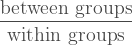
That’s unfortunate but considering what would happen if we knew that the length of side a is very illustrative. If the hypotenuse was exactly equal to 2 we knew that we could solve the entire triangle! Why? Consider again the value which we calculated which was 0.84r. That 0.84 is constant, only the r can vary as the size of the triangle increases or decreases.

In other words . . .

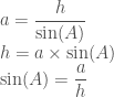
So if the angle A 1 and the length of the corresponding side is 2. . .

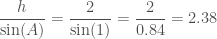
This is where the identities taught to school children as “sine equals opposite over hypotenuse” and “cosine equals adjacent over hypotenuse” come from. Intuitively if the length of the sides is determined by the hypotenuse and the angle then the angle must be determined by the hypotenuse and the sides!

Next up is the tangent function!

Code for drawing the sine and cosine. The circ() function is not from base R, we created last time.

circ(xlim = c(-1.5,1.5), ylim = c(-1.5,1.5), lwd = 1, 
	main = 'Unit Circle With Sine and Cosine')
segments(0, 0, cos(1), sin(1), lwd = 2)
text(.20, .45, 'Radius', srt = 57)
lines(th, lwd = 1.5)
text(.17, .1, expression(theta))
segments(0, 0, cos(1), 0, lwd = 2, col = 'blue')
text(.3, -.05, 'Cos', col = 'blue')
segments(cos(1), sin(1), cos(1), 0, lwd = 2,col = 'darkorchid')
text(.65, .3, 'Sin', col = 'darkorchid')

Drawing the triangle to solve. Basically the same shape with different labels.

segments(0, 0, cos(1), sin(1), lwd = 2)
segments(cos(1), sin(1), cos(1), 0, lwd = 2)
segments(0, 0, cos(1), 0, lwd = 2)

text(.1, 0.07, 'A')
text(cos(1)+.07, sin(1)/2, 'a')
text(cos(1)/2, -0.07, 'b')
text(cos(1)-.04, sin(1)-.15, 'B')
text(cos(1)/3, .4, 'h')

rect(cos(1)-.1,0,cos(1),.1)

The Circle – Taking a Walk

In this post we will take a walk on the unit circle. The unit circle is a circle with a radius of 1 arbitrary unit. Exploration of circles is usually done on the unit circle because it simplifies all sorts of math.

To begin with let us define precisely what a circle is: It is the set of all points which are the same distance from a point called the center. The area within a circle is called a disc. Traditionally we describe the unit circle as existing in R² space so each point has the coordinates (x,y).

Let’s attempt the simple task of drawing a circle.

The unit circle has a radius of 1.

The normal unit circle is centered at the point (0,0) called the origin. If it is centered elsewhere we write it as (a,b).

According to the definition of a circle that is sufficient information so lets take a look at the origin point, the radius, and the circle itself. I’ll draw it quickly and then we can try to study it.

Now let’s see what we can figure out immediately about this shape.

Obviously . . .

. . . and . . .

That is sufficient to draw four points, two on each axis.

There are an infinite number of points, though, so we will have to pick up the pace considerably if we ever want to finish this thing. Let’s try to evaluate the point x=0.5 and see what we can learn. Since the circle is described by the radius the position of (x=0.5,y=?) is the point where the tip of the radius line touches x=0.5.

That looks like a right triangle to me! We know two of the sides, the radius is the hypotenuse and the short side is 0.5 because we decided it would be. The old Pythagorean theorem tells us how to solve this

. . . thus . . .

. . . thus . . .

. . . thus . . .

. . . thus . . .

And since every point is related to the center in the same way, by the definition of the circle, we can now solve for every point.

In R we can write this as:

## The radius
r <- 1
## Sequence of x-values
x <- seq(-1,1,.01)
## The equation that defines y
y <- sqrt(r^2 - x^2)

## Since we need the positive and negative
## values of y at each x we do a little more.
x <- c(x,x)
y <- c(y,-y)

# Plot it.
plot(y~x, asp = 1)

You can see that the point’s we’ve plotted aren’t evenly spaced but they do describe a circle.

The fact that the unit circle, and thus any circle, is “solved” by the Pythagorean theorem, which we normally associate with triangles, is critically important. Much of our basic knowledge of these two shapes comes from their relationship.

The simplest way to draw a circle is to use Euler’s identity. The function only asks us for the angle associated with each point. We’ll come back to this function later on when we look at Euler’s identity. For now feel free to try it out and see that it works.

circ <- function(th = 2*pi, shift = 0, scale = 1, n = 99,
			xlim = c(-1,1), ylim = c(-1,1), lwd = 2,
			xlab = 'x', ylab = 'y', main = '', draw = TRUE){
	th <- seq(0,th,len=(n+1))+shift
	z <- exp(1i*th) * scale
	x <- Re(z)
	y <- Im(z)
	out <- data.frame(x,y)

	if(draw == TRUE) {
	plot(z, type = 'l', 
		lwd = lwd, asp = 1,
		xlab = xlab, ylab = ylab,
		xlim = xlim, ylim = ylim,
		main = main)
	}
	invisible(out)
}

## The drawings from this post.
circ(main = 'The Unit Circle')

circ(main = 'The Unit Circle \n With Points')
points(c(0,-1,0,1), c(1,0,-1,0), cex = 1.5, pch = 16)

circ(main = 'The Unit Circle \n With One Point')
segments(0,0,.5,.866)
segments(.5,.866,.5,0)
segments(0,0,.5,0)
text(.75,.9,label = '(x=0.5,y=??)')

The Circle – Radians

In our last post we looked at degrees, the best known way of measuring an angle. In mathematics and engineering, however, the most popular method is to use radians. So what are radians and why do people use them instead of degrees?

Consider the unit circle with a radius of 1 unit. An angle of one radian describes an arc equal to the radius.

Turning to a more mathematical approach for a bit let’s look at the equation that defines the famous number π and quickly derive the concept of the radian with some simple equations.

. . . thus . . .

. . . thus . . .

Thus a radian is the unit of angle for which an entire circle comes to 2π units. At first this seems absurdly arbitrary but it is really exactly the opposite since the radian is defined in terms of the radius of the circle, hence the name. There are 2π radians in a circle because a circle has a circumference 2π times its radius. Being built directly from the fundamental properties of the circle it makes equations involving angles and circles much simpler. Trigonometry in particular involves radians very naturally.

More generally we can say that . . .

. . . where θ is an angle in radians, s is the length of the arc, and r is the radius of the circle. I prefer a slightly different characterization that comes from rearranging the terms of the equation . . .

. . . the length of the arc is the radius multiplied by the angle. It’s just that changing the length of an arc is easier for me to intuit than the size of an angle.

Since radians and degrees describe the same thing it is possible to convert between them. There are 360 degrees or 2π radians in a circle. The conversion, simplified, is then . . .

. . . and . . .

Many popular angles have neat presentations in radian form so long as you’re comfortable with having π in the definition. Charts exist to “help” convert between degrees and radians in your head but they’re messy. Instead just recognize that a right angle is π/2 radians and compare. This method goes back as far as Euclid who used the quad as a preferred measure of an angle so that he compared everything to right angles.

But we still haven’t established exactly why anyone should care about radians other than for calculating arcs. Having learned about degrees from an early age they seem easy to use and simple to understand while radians involve transcendental numbers. The problem with degrees is that they have no actual relation to circles whereas we’ve seen that radians are derived directly from the properties of the circle itself. Consequently formulas involving geometry written in degrees are almost impossible to read while ones written in radians are quite neat and important relationships between things are exposed.

In our next post we’ll look at the trigonometric functions and see how much easier radians are. In fact to write formulas in degrees we basically have to convert degrees to radians anyway.

Before we go it is worth being aware of some of the alternatives to degrees and radians:
The turn</strong (or full turn) is a complete turn around the circle. So a right angle is ¼ turn. The turn is conceptually simple but it lacks a number of important properties that make the radian so attractive.

The grad is an attempt at a metricated degree. The circle is first divided into four parts and those parts each in 100 gradians. The unit has not seen much use as it isn’t really an improvement on the degree and has none of the properties of the radian of turn.

The mil, which is equal to 1/1000 of a radian, should be familiar to people who use firearms. It is the standard NATO measure because scouts and snipers are often concerned with extremely small angles. The mil is used to quickly estimate size and distance of objects if you know one or the other. Unfortunately the mil isn’t quite standardized. NATO defines it as 1/6400 of a circle even though mathematically it is closer to 1/6283.

The Circle – Degrees

The degree is the measure of an angle that most people are familiar with. There are 360 degrees in a circle, which is another way of saying that a degree is 1/360th of a rotation around the circle. The degree symbol is a small circle.

No one is exactly certain who chose to set the degree to 1/360th of a circle or why. We should note that there is no good mathematical justification for doing so, it is mainly a matter tradition. However because it is tradition most people have a sense of intuition for the behavior of angles in degrees and think in them easily. By the time most people graduate high school they’re familiar with at least a few important angles.

The 90 angle is called the “right” angle and noted with a square angle marking.

45 degrees is half of 90 degrees.

It is often pointed out that 360 is a highly composite number, which is to say that no smaller number has more divisors than it (360 is divisible by, deep breath . . . 1, 2, 3, 4, 5, 6, 8, 9, 10, 12, 15, 18, 20, 24, 30, 36, 40, 45, 60, 72, 90, 120, 180, and 360). You can seen in this list that 360 is divisible by everything from 1 to 10 except 7 which helps significantly with having divisions that seem immediately natural to most people. The smallest number divisible by all of the numbers from 1 to 10 is 2520 so 360 is a reasonable compromise.

Degrees are sometimes further subdivded into minutes (1/60 of a degree) and seconds (1/60 of a minute or 1/360 of a degree). Minutes are marked with a ‘ symbol and seconds with a ” symbol. For example:

latex$ 120.71^\circ = 120^\circ \, 42^\prime \, 36^{\prime\prime} &s=1$

At the end of the day, however, it is difficult to work degrees and their subdivisions when doing most mathematics. Other measures, ones related to the actual properties of circles are used instead.

Just for fun we’ll use R to prove that the smallest number divisible by all the numbers from 1 to 10 is, in fact, 2520. In order to end up with a tractable program we must first collect our prior knowledge.

Firstly: Whatever the number is it must be a multiple of ten so if we only check every tenth number we don’t risk missing anything.
Secondly: It can’t be less than ten so we can start there.
Thirdly: We don’t have to check divisibility by one.
Fourthly: We don’t have to check divisibility by five.
Fifthly: If we check divisibility by 6, 7, 8, and 9 we don’t have to check divisibility by 2, 3 or 4.

divisibleByAll <- function(max.val,n=1000000,quiet=T) {
	
	a <- seq(max.val,n,max.val)
	lower <- ceiling(max.val/2)
	upper <- max.val-1
	for (i in lower:upper) {
		a <- a[a%%i==0]
	}
	a <- a[a!=0]
	if(quiet) {out <- list(smallest = a[1])}
	if(!quiet) {out <- list(smallest = a[1],all.checked=a)}
	out
}

We can use this functions to calculate the smallest number divisible by everything from 1 to x for the first sixteen numbers (I’d go higher but my computer is too slow).

x <- 1:16
y <- sapply(x,divisibleByAll)
y <- as.numeric(do.call('c',y))
data.frame(y)
        y
1      NA
2       2
3       6
4      12
5      60
6      60
7     420
8     840
9    2520
10   2520
11  27720
12  27720
13 360360
14 360360
15 360360
16 720720

As you can see it rises very quickly and stalls in a couple of places and, indeed, the smallest number which is divisible by one through nine is 2520.

ANOVA

An analysis of variance is a very common statistical test, although one which answers such a non-specific question that it can seem surprising that it is used at all. The null hypothesis which an ANOVA addresses is . . .

. . . “is the mean of every group the same?”

The alternative hypothesis is that at least one of the means is different.

It is called the analysis of variance because it compares within group variability to between group variability.

Like Ronald Fisher we will look at the iris data as an illustrative example. In this case we will use the petal lengths. Before we start let’s look at the output R gives us for an ANOVA of the data. As we examine the logic of the ANOVA we will come back to this output and see where each piece comes from.

options(show.signif.stars=F)
mod <- aov(iris$Petal.Length~iris$Species)
summary(mod)
              Df Sum Sq Mean Sq F value Pr(>F)
iris$Species   2  437.1  218.55    1180 <2e-16
Residuals    147   27.2    0.19

Okay now the logic step by step. The first thing to check should be if the means are generally close together.

The grand mean of the data is . . .

mean(iris$Petal.Length)
 3.758

. . . and the group means are . . .

with(iris, tapply(Petal.Length, Species, mean))
    setosa versicolor  virginica 
     1.462      4.260      5.552 

They’re not really clustered but surely this is the kind of thing which might occasionally occur by accident just due to natural variability. What we need from the ANOVA is a way to quantify this tendency.

In order to describe the between total variability we will compute the sum of squares . . .

sum.squares <- function(x) {
	a <- mean(x)
	b <- (a-x)^2
	out <- sum(b)
	out
}

You should recognize this process of taking the difference between the mean and each data point, squaring it, and summing the result as part of the calculation of the variance. The SS and variance are, in fact, near relatives. The SS is a way of looking at the variability. It happens that we can partition the SS in a way that we cannot do with the the raw differences so this will make our work easier in the future.

The total sum of squares . . .

tot.SS <- sum.squares(iris$Petal.Length)
round(tot.SS,3)
 464.325

. . . and we will do the same thing to find the within group sum of squares . . .

in.SS <- with(iris, tapply(Petal.Length, Species, sum.squares))
round(in.SS,3)
    setosa versicolor  virginica 
     1.478     10.820     14.925

We can see why Fisher chose this example, it is very good for an analysis of variance because the total SS of squares is obviously much larger than the within groups SS (and thus the between groups variance will be as well).

Adding up the SS within each group tells is the total within groups SS. Then we can subtract that from the total SS to see how much comes from differences between the groups.

round(sum(in.SS),3)
 27.223

between.SS <- tot.SS - sum(in.SS)
round(between.SS,3)
 437.103

So far everything we’ve done should be easy to follow, we’re just computing the SS and then cutting it up into pieces (something we can only do with the SS). Nonetheless, it might be easier to follow as a table.

Compare this table of SS to the output of the ANOVA we looked at, at the beginning. The within and between SS values are are exactly the ones it reported.

Now let’s consider the more specific logic of the ANOVA. What would this table look like if the null hypothesis were true?

The between groups SS should be close to zero. If all of the means are the same then the main source of variability would be whatever variability there is within groups. In other words when the null hypothesis is true the within groups SS should tend to be about the same as the total SS.

We’ve seen that we can think of the total SS as coming from two sources (within and between groups) so to answer the question of the ANOVA – Is there at least one difference? – we only need to compare those sources. In other words we should test how much variance is caused by the two sources. That is a fraction.

What to compare it to?

Well we have seen before that chi-squared distribution INSERT LINK is what happens with the sum of the squares of multiple normal distributions. Since one of the assumptions of the ANOVA is that the errors are normally distributed there must be a connection. Indeed we will compare the fraction above to the F-distribution, which is the ratio of two (scaled) chi-squared distributions.

. . . where U₁ and U₂ have degrees of freedom d₁ and d₂ respectively.

In order to scale the F distribution and out description of the data we need to know the degrees of freedom. Within groups there are 2 degrees of freedom and between groups there are 147.

Why are these the degrees of freedom? Degrees of freedom are the number of “free” values in the calculation. Since there are 150 data points and the total SS is fixed the total degrees of freedom is 149, since we could thus determine 150th value using the other 149. Then for the within groups SS is are just 2 degrees of freedom since there are 3 groups we know the within groups SS (same logic). All of the remaining degrees of freedom, then, go to the between groups SS.

This is everything we need to know!

(between.SS/2)/(sum(in.SS)/147)
 1180.161

This is our F-statistic (or f-value) and it says that 1180 times as much variability was between groups as within groups. Give that we are modeling compared to the F-distribution lets look at exactly where we are on the F-distribution (also because its funny) . . .

x <- seq(0,1500,.1) 
y <- df(x,147,2)
plot(y~x,type='l')
arrows(1180,.0125,1180,.1,code=1,angle=30,lwd=2,col='red')
text(1180,.125,'You Are Here',col='red')

The distribution goes off to infinity, of course, we’re just showing a segment of it that helps to highlight just how extreme our result is.

Calculating the exact p-value (the probability of getting a greater result) is just a matter of taking an integral of the probability from 0 to 1180 on this distribution. Doing this precisely is not easy. We can’t estimate “by hand” with summation and even the built in integrate() function that R has lacks the needed precision.

In any even the p-value is extremely low. The aov() function estimates it as less than . . .

. . . which is very small indeed.

To finish up let’s take one last look again at the ANOVA table that R calculated for us. We should understand everything involved.

options(show.signif.stars=F)
mod <- aov(iris$Petal.Length~iris$Species)
summary(mod)
              Df Sum Sq Mean Sq F value Pr(>F)
iris$Species   2  437.1  218.55    1180 <2e-16
Residuals    147   27.2    0.19

We know where the degrees of freedom come from. We understand the sum of squares, the F-value, and the p-value. The only thing we didn’t cover directly was the mean squares. Those are just the SS divided by the degrees of freedom.

Sum of Squares

Let’s look at partitioning the concepts of the sum of squares (or the sum of squared errors) as it is a principle that underlies a number of common statistical tests like the ANOVA, linear regression, and the chi-squared test.

The important principle that underlies the way we use the sum of squares is that if all of the data comes from the same distributions the total sum of squares and the sum of the sum of squares for each group will be the same. This is true but not trivial to prove.

Instead let’s look at it in action.

The sum of squares is defined as . . .

First some random data from a normal distribution . . .

x <- rnorm(2000)

Now we will use some R code to see what happens.

sum.squares <- function(x) {
	sum((x-mean(x))^2)
}

## The SS for each of four partitions
s1 <- sum.squares(x[1:500])
s2 <- sum.squares(x[501:1000])
s3 <- sum.squares(x[1001:1500])
s4 <- sum.squares(x[1501:2000])

## The SS for all of the data.
a <- sum.squares(x)
## Sum of the SS that comes from the partitions.
b <- sum(s1,s2,s3,s4)
a
 504.8449
b
 504.3293
a/b
 1.001022

Yep, the partitioned SS add up to the total SS.

This trait is not unique to the sum of squares. The sum of the absolute errors also has this trait.

sum.abs <- function(x) {
	sum(abs(x-mean(x)))
}

m1 <- sum.abs(x[1:500])
m2 <- sum.abs(x[501:1000])
m3 <- sum.abs(x[1001:1500])
m4 <- sum.abs(x[1501:2000])

a <- sum.abs(x)
b <- sum(m1,m2,m3,m4)
a
 170.3583
b
 170.1077
a/b
 1.001473

Since the absolute value is conceptually simpler than the square it seems like we should just be using the sum of absolutes in the ANOVA but we don’t. Why?

Like many instances of squares in statistics we do this because it makes finding analytic solutions to various problems much easier. The chi-squared distribution exactly describes the distribution of the sum of squares from one or more standard normal distribution.

(Since the standard normal distribution has a mean of zero we don’t have to write the subtraction.)

We can generate its approximate shape easily from some random variables.

e <- rnorm(10000)
f <- rnorm(10000)
g <- rnorm(10000)
s <- e^2+f^2+g^2

d <- data.frame(e,f,g,s)
round(head(d),2)
      e     f     g    s
1  0.58  1.55  0.24 2.79
2  0.19 -0.53 -1.05 1.42
3 -1.27 -0.58 -0.26 2.00
4 -1.02  0.05  1.90 4.66
5  1.08  0.09  0.41 1.35
6 -0.07  0.02 -0.28 0.08

x <- seq(0,10,.1)
y <- dchisq(x,3)
plot(density(s, cut = 0), xlim = c(0,10))
lines(x,y,
	col = 'red',
	lty = 'dashed', lwd = 2)

We already saw the chi-squared distribution once as part of deriving the t-test. We’ll see it again next time when we look at the ANOVA.

The Rank Sum Test

Last time we were looking at the ranks of the differences as part of a paired samples test. This time we will look at the ranks of the raw data. The first thing to do is arrange our data.

## The data
x <- c(3,1,5,8,2)
y <- c(1,2,11,4,10)

## As a single group.
v <- c(x,y)

## Names to keep track of the groups
gr <- c(rep('a',5),rep('b',5))

## Rank the data.
r <- rank(dat)

dat <- data.frame(gr,v,r)
dat
   gr  v    r
1   a  3  5.0
2   a  1  1.5
3   a  5  7.0
4   a  8  8.0
5   a  2  3.5
6   b  1  1.5
7   b  2  3.5
8   b 11 10.0
9   b  4  6.0
10  b 10  9.0

Now we sum the ranks of each group.

tapply(dat$r,dat$gr,sum)
 a  b 
25 30

Group a sums to 25 while group b sums to 30. We don’t look at the distribution of the ranks directly like we did with the Signed Rank test. Instead we will look at the U-distribution.

. . . where n is the number of sample in reach group and R is the sum of ranks for one of the groups. So for group a our sample values of U is . . .

This distribution is defined by the dwilcox() function that comes built in to R.

x <- 0:25
y <- dwilcox(x,5,5)
plot(y~x,type='h')

Like with every other traditional hypothesis test we’ve seen the test itself just involves looking at where we are on the relevant distribution. Again like the signed-rank test the relevant distribution is approaching a normal distribution.

Wilcoxon Signed-Rank Test

The Wilcoxon Rank Sum Test

Because the t-test is sensitive to violations of normality people have sought improvements on it for a long time. The most popular of these robust options is the Wilcoxon Rank Sum Test and the Wilcoxon Signed-Rank Test, the rank sum test is also known as the Mann-Whitney U Test.

In R we can use the Wilcoxon test with the wilcox.test() function.

The logic of the test is incredibly simple: If there is an difference between groups then one group will tend to have greater values than the other.

For the simplest case, with paired data, the signed-tank test can be used. We have two vectors, x and y, from which we will make a vector of differences called w.

x <- c(3,1,5,8,2)
y <- c(1,2,11,4,10)
w <- x-y

wilcox <- data.frame(x,y,w)
wilcox
  x  y  w
1 3  1  2
2 1  2 -1
3 5 11 -6
4 8  4  4
5 2 10 -8

Now, we will rank each element of w by its absolute value, so the largest difference is 8 on line five.

## Notice that the rank() function returns
## the ranks but doesn't sort the data.
rank(abs(w))
 2 1 4 3 5

wilcox$r <- rank(abs(w))
wilcox
  x  y  w r
1 3  1  2 2
2 1  2 -1 1
3 5 11 -6 4
4 8  4  4 3
5 2 10 -8 5

Next we sum up the ranks of where w is positive and a sum the ranks were w is negative. This results in two numbers W₊ and W_–.

Wp <- 2+3
Wn <- 1+4+5

The question becomes, what is the probability of getting each of those numbers randomly? Answering this question is how we construct the distribution that the test uses.

There were the simplest non-trivial case is to imagine that there were three pairs of data points, which means there are eight possible permutations for the sums. The greatest possible value for W₊ is 6 and smallest possible value is 0. The same is true of W_–. Let us consider a few cases.

How many ways can we get W₊ = 6? Only one, if all of the differences are positive. The sum of the positive ranks would be 1+2+3 = 6.

How many ways can we get W₊ = 5? Again, just one. The only arrangement that works for the smallest difference to be negative and the 2nd and 3rd positive because 2+3 = 5.

How many ways can we get W₊ = 4? Yes, again, only one arrangement works. If the 1st and 3rd rank are positive.

How many ways can we get W₊ = 3? There are two! Either the 1st and 2nd might be positive (1+2 = 3) or only the third rank might be positive (3 = 3).

For each the possible sums 2 through 0 is are again only one possible arrangement.

The distribution we end up with for this case is a somewhat silly looking probability mass:

comb <- 0:6
p <- dsignrank(comb,3)

plot(p~comb,
	type='h',ylim=c(0,max(p)),lwd=3,
	ylab='Probability',xlab='Sum',
	main='Signed Rank Distribution for N=3')

This can be generalized for an arbitrarily large number of pairs:

n <- 15
s <- sum(1:n)
comb <- 0:s

main <- paste0('Signed Rank Distribution for N=',n)

p <- dsignrank(comb,n)

plot(p~comb,
	type='h',ylim=c(0,max(p)),lwd=3,
	ylab='Probability',xlab='Sum',
	main=main)

Notice that for N = 15 the distribution is distinctly bell shaped. In fact it is approaching a normal distribution. This is fortunate for two reasons: Firstly it is exhausting to calculate the Wilcoxon distribution (even for a computer) and secondly the normal approximation performs somewhat better in cases where some values have the same rank since the exact value becomes slightly conservative.