One of the distributions that is most commonly defined as approximately normal is the t-distribution. It looks like this and is defined by only a single parameter, the degrees of freedom (called nu or υ).

The peak of the t-distribution is slightly lower than the peak of the normal distribution. If we adjust the parameter of the t-distribution, to reflect a large sample size, they become more similar. The peak rises and the tails get thinner. Here we compare a normal distribution and two different t-distributions.
So why do t-distributions exist?
t is a random variable distributed as . . .
. . . where Z is the standard normal and U is chi-squared distribution with r degrees of freedom.

Where did this come from? Far too few people ask this question.
Let’s compare it to an equation from the central limit theorem which describes how the sample means from a normally distributed population are distributed.

The similarity should be apparent but we can make it even more obvious by rewriting the definition of the t-distribution.
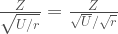
That’s right while the Z distribution is based on the mean and the standard deviation the t-distribution is based on the distribution of the mean and the distribution of the standard deviation. This is a perfectly sensible thing to want to describe when the mean and standard deviation aren’t known.
Why are we using the chi-squared, though? The chi-squared is naturally proportional the distribution of the variance of normally distributed data because it is based on the sum of squares of normal distributions and the variance is based on the mean of squares. Since the square root of the variance is the standard deviation the square root of the chi-squared is proportional to the standard deviation.
The first thing Gosset did for us was calculate exactly what that distribution is. Turns out it’s a real monster:

This uses the gamma function, which we haven’t studied yet, but that’s okay because we won’t be doing anything with this monstrosity of an equation except to acknowledge it. Historically people looked up needed information about the t-distributions on tables but today R can get us very precise values with the dt() family of functions.
The second thing Gosset did for us was find another equation that describes the behavior of the random variable t.
. . . thus we can cancel the (n-1) terms . . .
. . . thus we can rewrite the square root of division . . .
. . . square roots undo squares . . .
. . . division by a fraction is multiplication by its reciprocal . . .
. . . cancel out sigma . . .
. . . multiply together . . .


This means that . . .

The t-distribution is the sampling distribution of a random value called t when the population is a normal distribution. t itself is defined as (xbar-mu)/(s/sqrt(n)). Notice two things about this: First that it is a form of normalization, something familiar, and second that it does not ask us to know the standard deviation of the population.
Using our knowledge of how t relates to the data and the population we can reasonably test hypotheses about the population mean (μ) using a sample from the population. Like with the binomial test and Z-test what we do is compare the value that we have to the distribution of possible values.
Tomorrow we will look at the how the test is used in practice.
It is important to remember that although we’re not using the normal distribution directly we are still assuming that the population is normally distributed in order to get that particular precise Z-distribution. When the population is significantly non-normal t will not be distributed the way that we see in the images above.
