An analysis of variance is a very common statistical test, although one which answers such a non-specific question that it can seem surprising that it is used at all. The null hypothesis which an ANOVA addresses is . . .
. . . “is the mean of every group the same?”

The alternative hypothesis is that at least one of the means is different.
It is called the analysis of variance because it compares within group variability to between group variability.
Like Ronald Fisher we will look at the iris data as an illustrative example. In this case we will use the petal lengths. Before we start let’s look at the output R gives us for an ANOVA of the data. As we examine the logic of the ANOVA we will come back to this output and see where each piece comes from.
options(show.signif.stars=F)
mod <- aov(iris$Petal.Length~iris$Species)
summary(mod)
              Df Sum Sq Mean Sq F value Pr(>F)
iris$Species   2  437.1  218.55    1180 <2e-16
Residuals    147   27.2    0.19
Okay now the logic step by step. The first thing to check should be if the means are generally close together.
The grand mean of the data is . . .
mean(iris$Petal.Length)
 3.758
. . . and the group means are . . .
with(iris, tapply(Petal.Length, Species, mean))
    setosa versicolor  virginica
     1.462      4.260      5.552
They’re not really clustered but surely this is the kind of thing which might occasionally occur by accident just due to natural variability. What we need from the ANOVA is a way to quantify this tendency.
In order to describe the between total variability we will compute the sum of squares . . .
sum.squares <- function(x) {
	a <- mean(x)
	b <- (a-x)^2
	out <- sum(b)
	out
}
You should recognize this process of taking the difference between the mean and each data point, squaring it, and summing the result as part of the calculation of the variance. The SS and variance are, in fact, near relatives. The SS is a way of looking at the variability. It happens that we can partition the SS in a way that we cannot do with the the raw differences so this will make our work easier in the future.
The total sum of squares . . .
tot.SS <- sum.squares(iris$Petal.Length)
round(tot.SS,3)
 464.325
. . . and we will do the same thing to find the within group sum of squares . . .
in.SS <- with(iris, tapply(Petal.Length, Species, sum.squares))
round(in.SS,3)
    setosa versicolor  virginica
     1.478     10.820     14.925
We can see why Fisher chose this example, it is very good for an analysis of variance because the total SS of squares is obviously much larger than the within groups SS (and thus the between groups variance will be as well).
Adding up the SS within each group tells is the total within groups SS. Then we can subtract that from the total SS to see how much comes from differences between the groups.
round(sum(in.SS),3)
 27.223

between.SS <- tot.SS - sum(in.SS)
round(between.SS,3)
 437.103
So far everything we’ve done should be easy to follow, we’re just computing the SS and then cutting it up into pieces (something we can only do with the SS). Nonetheless, it might be easier to follow as a table.
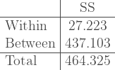
Compare this table of SS to the output of the ANOVA we looked at, at the beginning. The within and between SS values are are exactly the ones it reported.
Now let’s consider the more specific logic of the ANOVA. What would this table look like if the null hypothesis were true?
The between groups SS should be close to zero. If all of the means are the same then the main source of variability would be whatever variability there is within groups. In other words when the null hypothesis is true the within groups SS should tend to be about the same as the total SS.
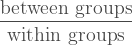
We’ve seen that we can think of the total SS as coming from two sources (within and between groups) so to answer the question of the ANOVA – Is there at least one difference? – we only need to compare those sources. In other words we should test how much variance is caused by the two sources. That is a fraction.
What to compare it to?
Well we have seen before that chi-squared distribution INSERT LINK is what happens with the sum of the squares of multiple normal distributions. Since one of the assumptions of the ANOVA is that the errors are normally distributed there must be a connection. Indeed we will compare the fraction above to the F-distribution, which is the ratio of two (scaled) chi-squared distributions.
. . . where U1 and U2 have degrees of freedom d1 and d2 respectively.

In order to scale the F distribution and out description of the data we need to know the degrees of freedom. Within groups there are 2 degrees of freedom and between groups there are 147.
Why are these the degrees of freedom? Degrees of freedom are the number of “free” values in the calculation. Since there are 150 data points and the total SS is fixed the total degrees of freedom is 149, since we could thus determine 150th value using the other 149. Then for the within groups SS is are just 2 degrees of freedom since there are 3 groups we know the within groups SS (same logic). All of the remaining degrees of freedom, then, go to the between groups SS.
This is everything we need to know!
(between.SS/2)/(sum(in.SS)/147)
 1180.161
This is our F-statistic (or f-value) and it says that 1180 times as much variability was between groups as within groups. Give that we are modeling compared to the F-distribution lets look at exactly where we are on the F-distribution (also because its funny) . . .
x <- seq(0,1500,.1)
y <- df(x,147,2)
plot(y~x,type='l')
arrows(1180,.0125,1180,.1,code=1,angle=30,lwd=2,col='red')
text(1180,.125,'You Are Here',col='red')

The distribution goes off to infinity, of course, we’re just showing a segment of it that helps to highlight just how extreme our result is.
Calculating the exact p-value (the probability of getting a greater result) is just a matter of taking an integral of the probability from 0 to 1180 on this distribution. Doing this precisely is not easy. We can’t estimate “by hand” with summation and even the built in integrate() function that R has lacks the needed precision.
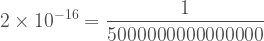
In any even the p-value is extremely low. The aov() function estimates it as less than . . .
. . . which is very small indeed.
To finish up let’s take one last look again at the ANOVA table that R calculated for us. We should understand everything involved.
options(show.signif.stars=F)
mod <- aov(iris$Petal.Length~iris$Species)
summary(mod)
              Df Sum Sq Mean Sq F value Pr(>F)
iris$Species   2  437.1  218.55    1180 <2e-16
Residuals    147   27.2    0.19
We know where the degrees of freedom come from. We understand the sum of squares, the F-value, and the p-value. The only thing we didn’t cover directly was the mean squares. Those are just the SS divided by the degrees of freedom.
