A while back we took a look at binomial tests. The two variations we looked at (one traditional and one Bayesian) were both single sample tests, they compared the behavior of the coin to that of a hypothetical coin with a known bias. In the field of making fair dice and fair coins this is a pretty reasonable test to do.
Often in science, however, we wish to compare two groups of samples. From a traditional perspective we wish to know if we can reasonably conclude they are drawn from differently shaped binomial distributions and from a Bayesian perspective we wish to describe the differences between groups.
There is no popular traditional test for this so instead we’ll just look at how to address the problem in terms of Bayesian estimation. To do so we have to introduce a technique called the Monte Carlo method, named after a large casino in Monte Carlo. Casinos make their money on statistics. Every game gives some edge to the house and when thousands of games are played that slight edge becomes a guaranteed source of income.
In statistics the Monte Carlo method is used to avoid having to do doing math! (Indeed much of the history of mathematics consists of brilliant thinkers trying to avoid mathematics.)
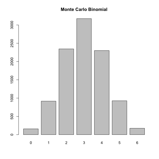
The Monte Carlo method works by producing large numbers of random values. For example we can generate a binomial distribution by flipping 6 coins ten thousand times and summing up the results.
barplot(table(colSums(replicate(10000,sample(c(0,1),6,replace=T)))))
Now let’s apply this to the question of comparing binomial data.
Recall that when we have binomial data in a Bayesian problem we use the Beta distribution to describe our knowledge about it. Last time we did this by using the dbeta() function to find where the density is. This time we will use the rbeta() function to produce a large number of values from the appropriate distribution.
Here is our information:
Our first coin flipped 100 heads and 50 tails.
Our second coin flipped 70 heads and 30 tails.
## Many random values from the distributions.
## We call each of them theta.
theta1 <- rbeta(10000,101,51)
theta2 <- rbeta(10000,71,31)

## The exact distributions.
comb <- seq(0,1,.01)
dens1 <- dbeta(comb,101,51)
dens2 <- dbeta(comb,71,31)

## Now let's compare the density to the sample.
par(mfrow=c(1,2))
plot(dens1~comb,xlim=c(.4,.8),type='l',lwd=2,main='Sample 1')
lines(density(theta1),col='red',lwd=2)
plot(dens2~comb,xlim=c(.5,.9),type='l',lwd=2,main='Sample 1')
lines(density(theta2),col='red',lwd=2)

Very similar, just as expected. If that isn’t close enough for your liking just increase the size of the sample.
Now we can make some simple inferences about the data. The quantile() function will produce a 95% interval and the median for each. Watch:
quantile(theta1,c(.025,.5,.975))
 2.5%   50% 97.5%
0.590 0.665 0.737

quantile(theta2,c(.025,.5,.975))
 2.5%   50% 97.5%
0.605 0.697 0.780
So 95% of the density of the first sample is between 0.590 and 0.737 (it is centered at 0.665).
I promised comparisons, though, and those turn out to be extremely easy to produce. The difference between theta1 and theta2 is . . . the difference between theta1 and theta2. This is why we needed to generate ten thousand random numbers rather than just looking at the density at each point.
diff <- theta1-theta2
quantile(diff,c(.025,.5,.975))
  2.5%    50%  97.5%
-0.145 -0.032  0.089
So there doesn’t seem to be much of a difference. The median difference is just -0.032, which is just about zero. Bayesian methods also allow us to visualize the distribution of results.
dth1 <- density(theta1)
dth2 <- density(theta2)
ddif <- density(diff)

r <- range(c(theta1,theta2))
y <- max(c(dth1$y,dth2$y))

par(mfrow=c(2,1))
plot(dth1,lwd=3,xlim=r,ylim=c(0,y),main='Thetas',col='blue')
lines(dth2,lwd=3,col='blue')
plot(ddif,col='turquoise',lwd=3,main='Difference')
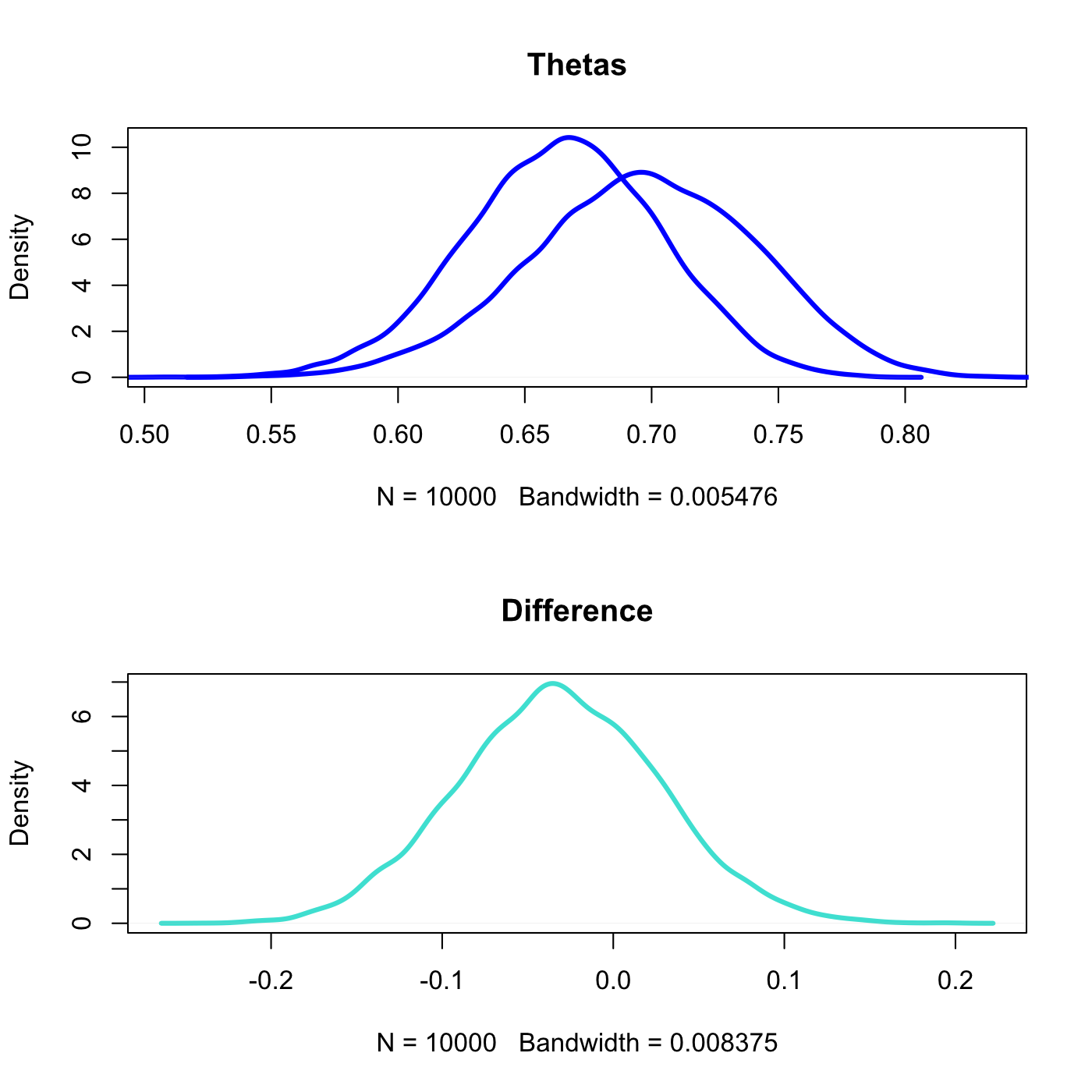
In blue we see the distribution of possible values for each coin’s bias. Below in turquoise are the distribution of differences.
