Multi-dimensional Distributions

The binomial distribution describes the probabilities that occur when “sampling with replacement” and the hypergeometric distribution describes the probabilities that occur when “sampling without replacement”. Both of them, however, are limited to the behavior of binary events like the flipping of a coin or success and failure. Extending them into multiple dimensions (and thus events that aren’t binary) requires understand exactly what the definitions of the basic distributions mean.

Before reading this post check the posts about the binomial coefficient, the binomial distribution, and the hypergeometric distribution to make sure you can follow along with the notation.

The multidimensional hypergeometric distribution is actually trivial. Let us make one change to how we define it. First there is N which is the population size and n which is the same size. Second there is K₁, the size of the first group, and k₁, the number we want from the first group along with K₂ and k₂ defined the same way along with K₃ and k₃ . . . and so on.

This is exactly the same as the equation for basic hypergeometric distribution, just parametrized differently. If we treat “success” and “failure” as simply two groups the equivalency is obvious:

In both cases we define how many ways there are to “correctly” pick from each group until we have all of the groups accounted for and multiply those combinations together then divide by the number of possible combinations.

Now for the binomial distribution. We took a look at where the defining equation comes from recently.

To see how this generalizes into multiple dimensions we start by expanding the binomial coefficient.

Now we will rename the parameters so that we can see what happens as the dimensions are added. Rather than defining “tails” in terms of “heads” (which is what is meant when we see n-k) everything gets its own name. Now there is n the sample size, k_x the number we want from each group, and p_x the probability of picking a each group.

It is then natural to see that the distribution generalizes in to multiple dimensions like this:

We can thus define sampling with replacement for any number of groups just by adding new terms as needed.

Binomial Distribution – Equation

Last time we looked at the binomial distribution it was purely to understand the behavior of a random variable. This time we’re going to look at the equation that defines it.

Here it is:

All of this notation should by now be familiar. The first part is a binomial coefficient and the rest is basic math. The variable n is the sample size and the variable p is the probability of success. Meanwhile k is the set of natural numbers N₀ (whole numbers from 0 to infinity). We test the probability at each value of k in order to create the distribution.

So why is this the equation?

I am not in the business of writing proofs, many good ones exist, but rather of producing intuition. The binomial coefficient is there because we are choosing from a set. It is there as a normalizing value to convert the rest of the equation into a meaningful probability.

Let us flips one coin three times. The probability that the coin will come up heads three times is p^3 since it has probability p each time. Alternatively the exponential term could be expanded to p*p*p. When we plug this into the equation:

Which can then be solved to become:

. . . which is . . .

. . . which is . . .

So it gives us the right answer.

How about the probability of getting two heads? The probability of getting heads twice is p^2 and the probability of getting one tails is (1-p)^1 so we multiply them together to find the probability. The result can be expanded to p*p*(1-p). This is not the probability of getting two heads and a tails, however, it is the total probability of getting each result.

What is the difference?

There are three equally likely ways to get this result so we have a probability of (p^2)*(1-p) three times! The equation is:

Which can then be solved to become:

Exactly what we predicted.

The Hypergeometric Distribution

This is a distribution you can impress your friend’s with because it has such an absolutely awesome sounding name and a comparatively simple form.

While the binomial distribution tells us about independent events the hypergeometric distribution tells us about a particular kind of dependent event, sampling without replacement. If you reach into a bag and take out a marble then reach in and take out another marble you are sampling without replacement. Like the binomial and Bernoulli distributions the hypergeometric describes events in terms of success and failure.

Here is our scenario in mathematical terms:

Randomly select n items from a set of N items. In this set there are K possible successes and N-K possible failures (which simply means everything is either a success of a failure). The probability of picking k successes from the set of K will follow the hypergeometric distribution. Which has this form:

Why? Let’s take a look.

Here is a random set from which we will pick three items. As per ancient statistical tradition consider it an urn containing while and black balls.

WBBBWBWBBWBBW

We will pick four balls from the urn and want to know how likely it is that exactly three of them will be black?

Here are our variables.

N = 13 # There are 13 items
K = 8  # 8 of them are black
n = 4  # We are selecting four items
k = 3  # Looking for 3 black

First we will describe how may ways there are to choose 3 black balls from a set of 8, because there are only 8 black balls in the set. Choose? That sounds like a binomial coefficient so let’s write _KC_k. Now how many ways are there to draw 1 white ball from a let of 5 white balls? That’s another binomial coefficient! We write it as _N-KC_n-k because N-K is the the number of non-black balls and n-k is the number of times we can pick a non-black ball.

Now we can simply multiply these together to get the number of correct combinations! There are 280 possible ways.

That’s not a probability, though, so we need to normalize it. How to do that? Well, how many ways are there to pick a combination from the set? That must be _NC_n since it is a set of N and we are choosing n items in total. That comes to 715.

So there are 280 correct results out of 715 total options. That’s just a fraction!

208/715
 0.3916084

There is a roughly 29% chance of us picking the particular combination of black and white balls that we want. And since we know that 280 is reakky _KC_k times _N-KC_n-k and that 715 is really _NC_n we can see where the equation comes from.

We can also summon up the hypergeometric distribution in R with the dhyper() family of functions.

dhyper(3,8,5,4)
 0.3916084

With so many variables there are tons of hypergeometric distributions but here’s a simple one that show the probability for between zero and four balls black chosen from an urn.

Successes <- 0:4
plot(dhyper(Successes,8,5,4)~Successes,
	type='h', lwd=3,
	ylim=c(0,.5), ylab='Probability',
	main='A Hypergeomatric Distribution')

Obviously the hypergeometric distribution is good for more than placing bets on Jacob Bernoulli’s less interesting party games or we wouldn’t be talking about it. The hypergeometric can be used to count cards. Perhaps most famously, however, it was used by Sir Ronald Fisher to devise a statistical test. He was given the task of testing the claim that fellow biologist Muriel Bristol-Roach could tell whether her tea was poured into the cup before the milk or after. The idea of the test was that distribution told him the best possible guesses that could be made for the experiment he designed.

Doctor Bristol-Roach was presented with eight cups of tea to taste, some poured milk first and some not. The lady then tasted them one-by-one reporting which type she believed each cup was. History records that the well bred biologist was more than validated by the experiment.

Binomial Coefficient

Binomial Coefficient

The binomial coefficient in probability theory, especially the study of discrete probabilities. It looks like this:

Because its notation is unfamiliar this can make otherwise comprehensible equation appear to be nonsense. Traditionally the binomial coefficient represents how many different ways you can pick k objects from a set of n objects. Consequently it is read as “n choose k”. This is why R uses the choose() function to denote it.

Let’s look at some examples

# How many ways to choose 5 from a set of 10?
choose(10,5)
 252
# How many ways to choose 3 from a set of 7?
choose(7,3)
 35

Outside of probability and statistics the binomial coefficient is sometimes written as _nC_k and is read the same way.

For pairs it is easy to represent every possible combination.

Lets look at ₅C₂ The easiest way to determine this by hand is to write out a triangle that contains every possible pairing. The first row is all of the pairings that contain a 1, there are four of these. Next is the pairings that contain a 2, there are also four of these but we already wrote the pairing 1-2 in the first row. Then the pairings that contains a 3, and then the ones that contain a 4. By the time we get to “all the pairings that contain a 5” there are none left, each of those pairs has already been written.

12, 13, 14, 15
23, 24, 25,
35, 34,
45

choose(5,2)
 10

How about more generally? Making a construct like this for something other than a pair isn’t nearly as easy. Also it takes more time.

The equation you will most often find that defines the binomial coefficient is n!/k!(n-k)! where the “!” symbol indicates the factorial operation rather than excitement. A factorial is a number multiplied by all of the smaller natural numbers. For example:

5*4*3*2*1
 120
factorial(5)
 120

Why does n!/k!(n-k)! produce the correct answer?

This is a question that has always bothered me because people tend not to explain so I’d like to present a simple proof of the equation that defines binomial coefficient. As you might have guessed I like to think in statistical terms so this proof will be based on probability, namely: What is the probability of picking any given combination? First notice that all combinations of the same size are equally likely so if we can find the probability of a given combination we know the probability of all of them.

Let’s say we want a combination of three letters from a set of nine, our target is to get A, B, and C.

## The first nine letters of the alphabet.
LETTERS[1:9]
[1] "A" "B" "C" "D" "E" "F" "G" "H" "I"

When we pick the first element there are 3 possible successes out of 9 (A or B or C, since order doesn’t matter). If we do pick correctly there are now 2 possible success out of 8 (since one of the correct letters is gone). Finally, if we pick correctly the second time there is 1 possible success out of 7.

Thus the probability of us drawing ABC, in some order, must be:

3/9 * 2/8 * 1/7
 0.0119047619 

That’s not very easy to read but fortunately the reciprocal will be. In fact it will tell us exactly the number of combinations.

1 / (3/9 * 2/8 * 1/7)
 84

Just to make sure I haven’t lead you down the garden path let’s check the respectable statistical software.

choose(9,3)
 84

Awesome!

The final steps are to consider what the equation 1 / (3/9 * 2/8 * 1/7) represents. In essence we’re flipping over all of those fractions. This means that we can extract the possible combinations in one step by just doing that.

9/3 * 8/2 * 7
 84

Now we will return to the forumula n!/k!(n-k)! and see how that excitable equation results in the equation we found. If we expand the factorial we get:

You may recall that in equations like this common terms “cancel out” and here you can distinctly see the ones that will. All that’s left is:

Quod Erat Demonstrandum

Bayesian Binomial Comparison

A while back we took a look at binomial tests. The two variations we looked at (one traditional and one Bayesian) were both single sample tests, they compared the behavior of the coin to that of a hypothetical coin with a known bias. In the field of making fair dice and fair coins this is a pretty reasonable test to do.

Often in science, however, we wish to compare two groups of samples. From a traditional perspective we wish to know if we can reasonably conclude they are drawn from differently shaped binomial distributions and from a Bayesian perspective we wish to describe the differences between groups.

There is no popular traditional test for this so instead we’ll just look at how to address the problem in terms of Bayesian estimation. To do so we have to introduce a technique called the Monte Carlo method, named after a large casino in Monte Carlo. Casinos make their money on statistics. Every game gives some edge to the house and when thousands of games are played that slight edge becomes a guaranteed source of income.

In statistics the Monte Carlo method is used to avoid having to do doing math! (Indeed much of the history of mathematics consists of brilliant thinkers trying to avoid mathematics.)

The Monte Carlo method works by producing large numbers of random values. For example we can generate a binomial distribution by flipping 6 coins ten thousand times and summing up the results.

barplot(table(colSums(replicate(10000,sample(c(0,1),6,replace=T)))))

Now let’s apply this to the question of comparing binomial data.

Recall that when we have binomial data in a Bayesian problem we use the Beta distribution to describe our knowledge about it. Last time we did this by using the dbeta() function to find where the density is. This time we will use the rbeta() function to produce a large number of values from the appropriate distribution.

Here is our information:
Our first coin flipped 100 heads and 50 tails.
Our second coin flipped 70 heads and 30 tails.

## Many random values from the distributions.
## We call each of them theta.
theta1 <- rbeta(10000,101,51)
theta2 <- rbeta(10000,71,31)

## The exact distributions.
comb <- seq(0,1,.01)
dens1 <- dbeta(comb,101,51)
dens2 <- dbeta(comb,71,31)

## Now let's compare the density to the sample.
par(mfrow=c(1,2))
plot(dens1~comb,xlim=c(.4,.8),type='l',lwd=2,main='Sample 1')
lines(density(theta1),col='red',lwd=2)
plot(dens2~comb,xlim=c(.5,.9),type='l',lwd=2,main='Sample 1')
lines(density(theta2),col='red',lwd=2)

Very similar, just as expected. If that isn’t close enough for your liking just increase the size of the sample.

Now we can make some simple inferences about the data. The quantile() function will produce a 95% interval and the median for each. Watch:

quantile(theta1,c(.025,.5,.975))
 2.5%   50% 97.5% 
0.590 0.665 0.737

quantile(theta2,c(.025,.5,.975))
 2.5%   50% 97.5% 
0.605 0.697 0.780

So 95% of the density of the first sample is between 0.590 and 0.737 (it is centered at 0.665).

I promised comparisons, though, and those turn out to be extremely easy to produce. The difference between theta1 and theta2 is . . . the difference between theta1 and theta2. This is why we needed to generate ten thousand random numbers rather than just looking at the density at each point.

diff <- theta1-theta2
quantile(diff,c(.025,.5,.975))
  2.5%    50%  97.5% 
-0.145 -0.032  0.089

So there doesn’t seem to be much of a difference. The median difference is just -0.032, which is just about zero. Bayesian methods also allow us to visualize the distribution of results.

dth1 <- density(theta1)
dth2 <- density(theta2)
ddif <- density(diff)

r <- range(c(theta1,theta2))
y <- max(c(dth1$y,dth2$y))

par(mfrow=c(2,1))
plot(dth1,lwd=3,xlim=r,ylim=c(0,y),main='Thetas',col='blue')
lines(dth2,lwd=3,col='blue')
plot(ddif,col='turquoise',lwd=3,main='Difference')

In blue we see the distribution of possible values for each coin’s bias. Below in turquoise are the distribution of differences.

Weird Facts from MTG JSON: Converted Mana Cost

Welcome back to my irregular series Weird Facts from MTG JSON, using data made available by Robert Shultz on his site.

In Magic: The Gathering every card requires a resource called “mana” in some amount in order to be used. The converted mana cost (abbreviated cmc) can be can zero or any natural number. Now we might wonder how those costs are distributed among the more than 13 thousand unique cards in the game.

Naively there are a lot of valid possibilities but anyone familiar with the game will be know that the vast majority of cards cost less than five mana. I expect they would be hard pressed to say with confidence which cost is the most common, though. Let’s check it out!

First the data itself:

library(rjson)
source("CardExtract.R")
## Read the data into R.
AllSets <- fromJSON(file="AllSets.json")

## Filter all of it through the extraction function,
## bind it together and fix the row names.
l <- lapply(AllSets,extract.cards)
AllCards <- AllCards[AllCards$exp.type != "un",]
AllCards <- do.call(rbind.data.frame,l)
rownames(AllCards) <- 1:length(AllCards$cmc)

Now we take three pieces of information we need, the name, the cost, and the layout for each card. We get rid of everything except “ordinary” cards and the squeeze out everything unique that remains so reprints don’t affect our results.

name <- AllCards$name
cmc <- AllCards$cmc
lay <- AllCards$layout
dat <- data.frame(name,cmc,lay)
dat <- dat[dat$lay == 'normal' | dat$lay == 'leveler',]
dat <- unique(dat)

Here’s where something very interesting happens so bear with me for a second. Let’s plot the counts for each unique cmc.

plot(table(dat$cmc),
	ylab='count',xlab='cmc',
	main='Costs of Magic Cards')

If you read Wednesday’s post where we recreated the London Blitz this should look very familiar. That’s right, the costs of Magic cards follow a Poisson distribution. We can add some points that show the appropriate Poisson distribution.

m <- mean(dat$cmc)
l <- length(dat$cmc)
comb <- 0:16
plot(table(dat$cmc),
	ylab='count',xlab='cmc',
	main='Costs of Magic Cards \n Poisson In Red')

Its a ridiculously good fit, almost perfect. What is going on exactly? I mean I doubt they did this deliberately. When we last saw the Poisson distribution, and in almost every explanation of it you will ever find, the Poisson is the result of pure randomness. Are the design and development teams working blindfolded?

(Image from “Look At Me I’m The DCI” provided by mtgimage.com)
(Art by Mark Rosewater, Head Designer of Magic: The Gathering)

Nope. The secret is to think about where exactly the Poisson distribution comes from and forget its association with randomness. It requires that only zero and the natural numbers be valid possibilities and that a well defined average exists. Although Magic has never had a card which cost more than 16 mana there’s no actual limitation in place, high costs are just progressively less likely.

I expect that what we are seeing here is that the developers have found that keeping the mean cost of cards at around 3.25, in any given set, makes for good gameplay in the Limited format. Because they also want to keep their options open in terms of costs, a creature that costs more than 8 mana is a special occasion, the inevitable result is a Poisson distribution.

The Volley Problem

Here’s a question for you. A line of musketeers, ten abreast, is firing on the enemy. Each man has a 10% chance of hitting his target at this range. What is the probability that at least one of them will hit in the first volley? This is a traditional sort of problem in logic and probability. To some people it seems as though there ought to be a 100% chance since that’s 10 times 10 but some further thought reveals that since there is some chance of each of them missing there must be some chance of all of them missing.

We calculate the result 100% minus the probability of each missing (90%) to the power of the number of musketeers (10).

1-(.9^10)
0.651

So about an 65% chance of at least one of them hitting.

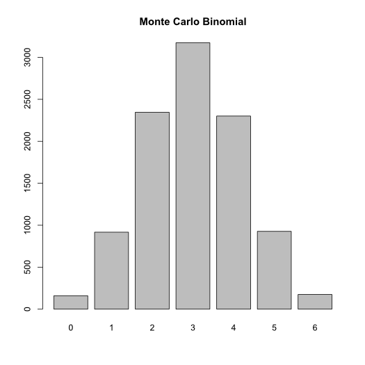
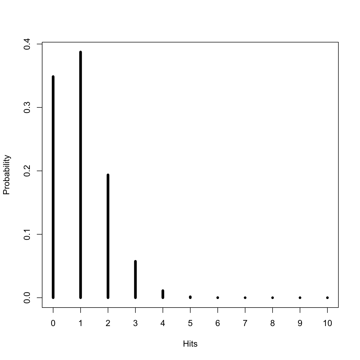
That’s not a super informative result since it doesn’t tell us anything like what the most likely number of hits is. Consider this however: Shooting at a target is a Bernoulli trial, just like the flipping of a coin. It has exactly two outcomes, hit or miss, and particular probability. Thus the successes of the musketeers ought be following a Binomial distribution (both logically and because I have a theme going). Indeed they do, the distribution of their volleys should look like this:

We see immediately that the most likely outcome is that 1 of them will hit and that is almost inconceivable that more than 4 of them will hit. Musketeers were not terrible efficient military machine, although they were quite deadly en masse.

Say you are the commander of this line and you’re not happy with the atrocious accuracy of these soldiers. You want a 90% of getting at least one hit. How much better do the musketeers have to be?

Thanks to computers the easiest method, and most general, is to just test many possible values.

## Many candidate values of q, the probability of a miss
q <- seq(.9,.5,-.01)
## The corresponding values of p.t the total probability 
## of a hit for the musketeers as a group.
p.t <- 1-(q^10)

## We set a equal to the smallest values of p.t that is equal
## to or greater than 0.9 and then check out what is on that
## line.
dat <- data.frame(q,p.t)
a <- min(dat$p.t[p.t >= .9])
dat[dat$p.t==a,]
      q         p.t
12 0.79 0.9053172

Recalling that for Bernoulli trials p = 1 – q we conclude that the probability of hitting on each shot it 0.21, or a 21% chance. The soldiers need to double their accuracy. You will also notice that if you make a binomial distribution with the new value of p the most likely outcome is now that two of the soldiers will hit.

For safety’s sake lets work out the analytical solution to the problem in order to check out answer.

.9 = 1-(x^10)
.9+(x^10) = 1
x^10 = .1
x = .1^.1
x = .794
1-.794
.206

Yep, that’s basically the same answer.

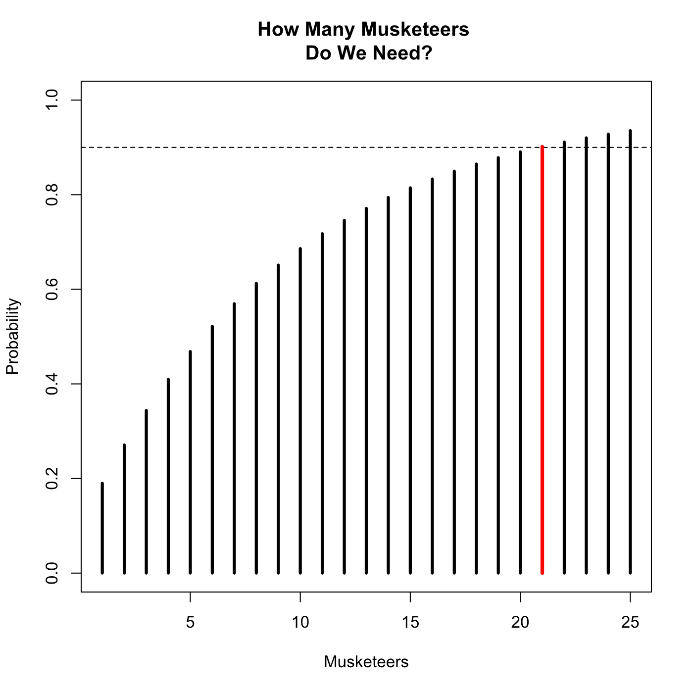
What if we tried to solve our problem the other way around? Historically musket lines were enormous and successful in part because it was easier to hand a musket to ten people than train one person to be a really good shot with them. How many musketeers need to be on the line to have a 90% that at least one of them will hit?

We could, of course, use the same method as we did before and simply recalculate for larger and larger numbers of musketeers. If we did we would end up with a cumulative geometric distribution a relative of the binomial.

Like the binomial the geometric distribution is discrete, it has values only at whole numbers.

If there is one musketeer there the probability of hitting is 0.100, if there are two the probability is 0.190 (not quite double), if there are three the probability is 0.271, and so on. Eventually, with 21 musketeers, the probability rises to fully 0.902 and we’re done.

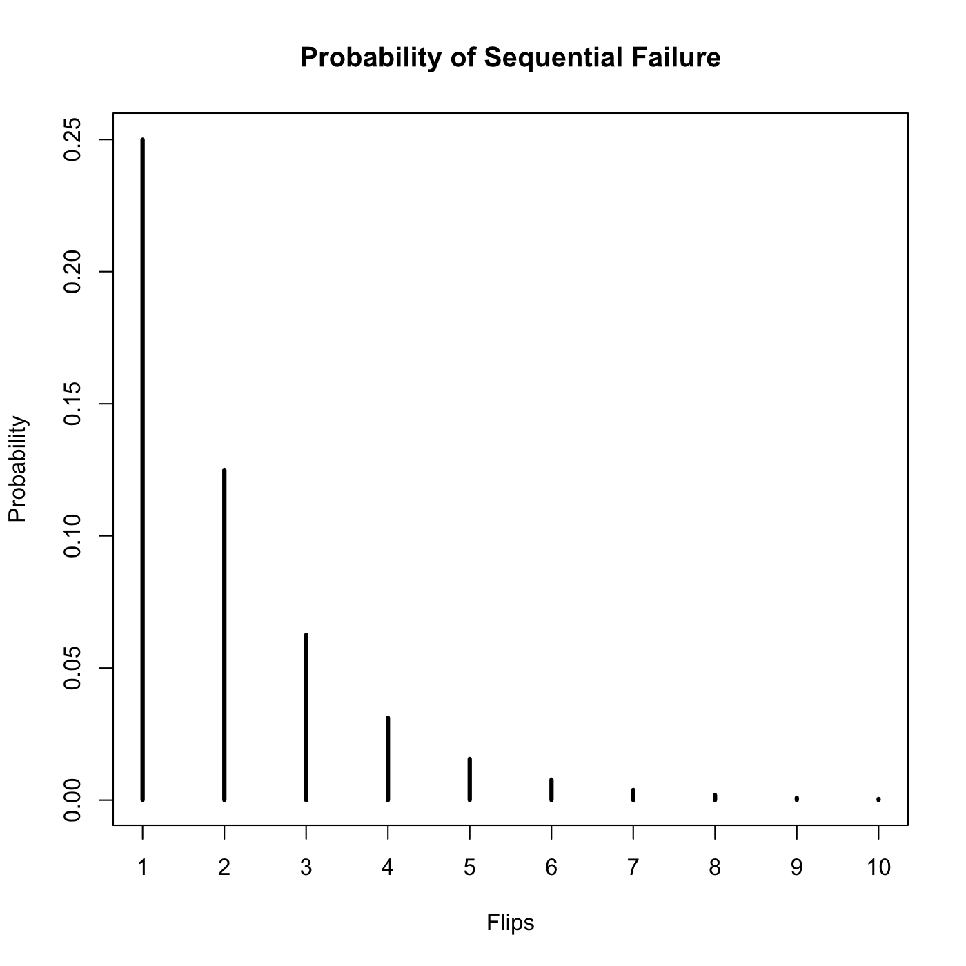
The plain geometric distribution itself is the probability that it will take N trials to get a success. Here is the flipping of a fair coin:

The probability of getting Tails on the first flip is 50%, the probability of getting Tails on the first flip and the second flip is 25%. This is why the cumulative distribution shows us the probability of getting a heads.

The code for our graphics in this post.

The binomial distribution. This is very simple but I include it because the xaxp argument is so rarely used. R creates tick marks automatically but not the ones I wanted in this case. The argument tells R the smallest tick mark to label, the largest one, and the total number of tick marks.

Hits <- 0:10
Probability <- dbinom(0:10,10,.1)
volley <- data.frame(Hits,Probability)

plot(volley,type='h',lwd=5,xaxp=c(0,10,10))

The cumulative geometric distribution.

## When the code \n is used in a string R will read it as creating a new line.
plot(pgeom(1:25,.1),type='h',lwd=3,
	main='How Many Musketeers \n Do We Need?',xlab='Musketeers',ylab='Probability',
	ylim=c(0,1))
## Create a horizontal dashed line.
abline(h=.9,lty=2)
## Draw a red line that covers column 21.
segments(21,0,21,0.9015229,col='red',lwd=3.5) 

The Poission Distribution

The Poisson Distribution

The Poisson distribution is actually based on a relatively simple line of thought. How many times can an event occur in a certain period?

Let’s say that on an average day the help center gets 4 calls. Sometimes more and sometimes less. At any given moment we can either get a call or not get a call. This tells us that the probability distribution which describes how many calls we are likely to get each day is Binomial. Furthermore we know that it must be of the form Binomial(N,4/N) where where N is the greatest possible number of calls because this is the only way for the mean to be 4.

The question now becomes how many call is it possible to get in a day? Hard to say but presumably the phone could be ringing off the hook constantly. Its outrageously unlikely for me to get a hundred calls in a day but there is some probability that everyone in the building could need help on the same day. It is rarely possible to set an upper limit with confidence but watch what happens as we make the limit higher and higher.

As we increase the The distribution is converging on a particular shape. Poisson proved what the shape would become if N were infinite. He also showed that this new distribution was much easier to calculate the form of than the Binomial distribution. Since a very large N and an infinite N are nearly identical the difference is irrelevant so long as its possible for the event to happen a large number of times.

Since the Poisson distribution is effectively a Binomial distribution with N always set to the same value we can describe the Poisson using only the average rate. Here it is for an average rate of 4 events per interval (calls per day, meteor strikes per year, etc).

It is occasionally said the the Poisson distribution is the “law of rare events” which is a sort of true but mostly confusing title. What matters is that the event could potentially happen much more often than it does.

A switchboard that gets an average of 100 calls an hour is not getting calls “rarely” but it is going to follow a Poisson distribution because a call can happen at any moment during the hour. If the switchboard were very slow and could only handle one call every ten seconds (so never more than 360 calls in an hour) it would be better to use a binomial distribution.

When explaining things it is often better to show than tell. Let’s look at an example of how the Poisson arises.

The Blitz was a massive bombing of Britain during World War II. A major concern of the British government was whether or not the Nazi bombs were precise weapons. If the bombs were guided their policies to protect people in the cities would have to be different. The analysts knew that if the bombing were random the distribution of bombs would have to follow an approximately Poisson distribution.

We can simulate a bombing campaign pretty easily by creating a large number of random coordinates to represent for each hit. The city is ten kilometers by ten kilometers.

set.seed(10201)
x <- runif(300,0,10)
y <- runif(300,0,10)
xy <- data.frame(x,y)

And what does this attack look like? We’ll plot each point and overlay a 10×10 grid.

p <- ggplot(xy,aes(x=x,y=y))
p + geom_point(size=2.5,color='red') +
	geom_hline(yintercept=0:10) +
	geom_vline(xintercept=0:10) +
	scale_x_continuous(minor_breaks=NULL,breaks=NULL) +
	scale_y_continuous(minor_breaks=NULL,breaks=NULL) +
	coord_cartesian(xlim=c(0,10),ylim=c(0,10))

During the Blitz each square had to be counted up by hand. We can do a little better. The cut() function divides up the data into one hundred sections then we rename them into something easier to read.

xx <- cut(x,10)
yy <- cut(y,10)
levels(xx) <- 1:10
levels(yy) <- 1:10

A contingency table tells now tells us how many bombs landed in each square. As a dataframe its easier to work with. Making a plot to see how often each number of its came up is then very simple.

fr <- data.frame(table(xx,yy))
plot(table(fr$Freq))

It isn’t a perfect, fit, of course, but as we discussed about the philosophy of statistics we do not expect perfection. The trend is one that clearly approximates the Poisson distribution.

Bernoulli Distribution

The Bernoulli Distribution

When we first started looking at statistical inference a few weeks ago the binomial distribution was introduced, which reflects the behavior of a coin that has been flipped many times. The Bernoulli distribution is simpler case which the binomial is a generalization of, it represent a coin flipped a single time.

Here’s an example for a biased coin:

bern <- data.frame(Value=c(0,1),Probability=c(.3,.7))

plot(bern,type='h',lwd=5,ylim=c(0,1),main="Bernoulli(0.3,0.7)")
points(bern,cex=2,pch=16) # Add large, solid color points

Obviously you can’t get a lot of mileage out of this distribution. It is, however, the source of a lot of common terminology in statistics. By tradition Heads = 1 and Tails = 0 (which part of the reason that in R and many other languages the logical values TRUE and FALSE equal 1 and 0, respectively). The probability of Heads is written p while the probability of tails is written q. Since a coin only has two sides it is always true that q = 1-p and p = 1-q.

Anything that has discrete “success” and “failure” modes can be considered a Bernoulli trial. Flipping a coin is a Bernoulli trial. Rolling a die is a Bernoulli trial if you define every face as either success of failure (ie “a 6 is a success” or “all odds are successes”). Some things are close enough to Bernoulli trial that they can generally be thought of in these terms, for example, many text books use the sex of a newborn as a an example of a Bernoulli trial even though about 1% of people are born with ambiguous or intersex characteristics.

Bernoulli’s name is also given to the concept of a Bernoulli process which is multiple, independent, identical Bernoulli trials. This means that this is more than one trial, trials have no effect on each other, and the probability of success is the same each time. This is what creates a binomial distribution (flipping a coin many times). On the other hand drawing black and white marbles from a box isn’t a Bernoulli process because once you take a black marble out the probability of drawing a black marble decreases, the trials are not identical.

Hypothesis Testing – A Warning

Consider the traditional binomial test for a moment. The goal is to decide whether or not the sample we have is reasonable based on our hypothesis. This is called a significance test.

There is a problem with this, however, namely that there is no subtlety in the hypothesis. If we hypothesize that a coin is fair we mean that the coin has a probability of 0.5 of heads. This is fine in the realm of pure mathematics but in reality it is always true that the null hypothesis is wrong. No coin will actually be perfectly fair but it may be extremely close to fair, so much that it is irrelevant.

Imagine a coin that flips heads with a probability of 0.495, which is quite good. The binomial test doesn’t care, though. For a small sample of rolls the binomial test lacks the sensitivity to notice that 0.495 is not 0.5 but as the sample gets larger the test becomes more sensitive. Eventually it will begin to notice even meaningless differences and report that it is improbable the die is fair.

We can actually watch this happen with a bit of R code. We will keep the same relative probability of heads as we increase the sample.

h <- 495*c(1,2,5,10,20)  #Number of heads
t <- 1000*c(1,2,5,10,20) #Total sample size

a <- binom.test(h[1],t[1])
b <- binom.test(h[2],t[2])
c <- binom.test(h[3],t[3])
d <- binom.test(h[4],t[4])
e <- binom.test(h[5],t[5])

# Extract the p-values as a vector then print them out to three decimal places for ease of reading.
round(as.numeric(c(a[3],b[3],c[3],d[3],e[3])),3)
[1] 0.776 0.671 0.488 0.322 0.159

With a sample of 1000 we are told that there is a 77.6% chance of getting so extreme a value. With a sample of 20000, though, the chance is just 15.9%. This is a result of the test working correctly but perhaps not intuitively.

With a huge sample the test is very sensitive, it becomes better at discriminating between the null hypothesis and the alternative. What the test does not do (and is not meant to do) is tell us whether the difference is large or meaningful. By taking an arbitrarily large sample we can guarantee that the p-value of the test will be low, no matter how close the coin is to being fair.

Be careful when interpreting p-values and keep an awareness of what they are and are not!