Multi-dimensional Distributions

The binomial distribution describes the probabilities that occur when “sampling with replacement” and the hypergeometric distribution describes the probabilities that occur when “sampling without replacement”. Both of them, however, are limited to the behavior of binary events like the flipping of a coin or success and failure. Extending them into multiple dimensions (and thus events that aren’t binary) requires understand exactly what the definitions of the basic distributions mean.

Before reading this post check the posts about the binomial coefficient, the binomial distribution, and the hypergeometric distribution to make sure you can follow along with the notation.

The multidimensional hypergeometric distribution is actually trivial. Let us make one change to how we define it. First there is N which is the population size and n which is the same size. Second there is K1, the size of the first group, and k1, the number we want from the first group along with K2 and k2 defined the same way along with K3 and k3 . . . and so on.

\displaystyle \frac{\binom{K_1}{k_1}\binom{K_2}{k_2}\binom{\cdots}{\cdots}\binom{K_x}{k_x}}{\binom{N}{n}}

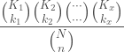
This is exactly the same as the equation for basic hypergeometric distribution, just parametrized differently. If we treat “success” and “failure” as simply two groups the equivalency is obvious:

\displaystyle \frac{\binom{K_1}{k_1}\binom{K_2}{k_2}}{\binom{N}{n}} = \frac{\binom{K}{k}\binom{N-K}{n-k}}{\binom{N}{n}}

In both cases we define how many ways there are to “correctly” pick from each group until we have all of the groups accounted for and multiply those combinations together then divide by the number of possible combinations.

Now for the binomial distribution. We took a look at where the defining equation comes from recently.

\displaystyle \binom{n}{k}p^k(1-p)^{n-k}

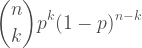
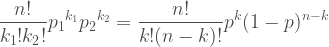
To see how this generalizes into multiple dimensions we start by expanding the binomial coefficient.

\displaystyle \frac{n!}{k!(n-k)!}p^k(1-p)^{n-k}

Now we will rename the parameters so that we can see what happens as the dimensions are added. Rather than defining “tails” in terms of “heads” (which is what is meant when we see n-k) everything gets its own name. Now there is n the sample size, kx the number we want from each group, and px the probability of picking a each group.

\displaystyle \frac{n!}{k_1!k_2!}{p_1}^{k_1}{p_2}^{k_2} = \frac{n!}{k!(n-k)!}p^k(1-p)^{n-k}

It is then natural to see that the distribution generalizes in to multiple dimensions like this:

\displaystyle \frac{n!}{k_1! k_2! \cdots k_x!} {p_1}^{k_1} {p_2}^{k_2} \cdots {p_x}^{k_x}

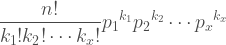
We can thus define sampling with replacement for any number of groups just by adding new terms as needed.

Binomial Coefficient

Binomial Coefficient

The binomial coefficient in probability theory, especially the study of discrete probabilities. It looks like this:

\displaystyle \binom{n}{k}

Because its notation is unfamiliar this can make otherwise comprehensible equation appear to be nonsense. Traditionally the binomial coefficient represents how many different ways you can pick k objects from a set of n objects. Consequently it is read as “n choose k”. This is why R uses the choose() function to denote it.

Let’s look at some examples

# How many ways to choose 5 from a set of 10?
choose(10,5)
 252
# How many ways to choose 3 from a set of 7?
choose(7,3)
 35

Outside of probability and statistics the binomial coefficient is sometimes written as nCk and is read the same way.

For pairs it is easy to represent every possible combination.

Lets look at 5C2 The easiest way to determine this by hand is to write out a triangle that contains every possible pairing. The first row is all of the pairings that contain a 1, there are four of these. Next is the pairings that contain a 2, there are also four of these but we already wrote the pairing 1-2 in the first row. Then the pairings that contains a 3, and then the ones that contain a 4. By the time we get to “all the pairings that contain a 5” there are none left, each of those pairs has already been written.

12, 13, 14, 15
23, 24, 25,
35, 34,
45

choose(5,2)
 10

How about more generally? Making a construct like this for something other than a pair isn’t nearly as easy. Also it takes more time.

The equation you will most often find that defines the binomial coefficient is n!/k!(n-k)! where the “!” symbol indicates the factorial operation rather than excitement. A factorial is a number multiplied by all of the smaller natural numbers. For example:

5*4*3*2*1
 120
factorial(5)
 120

Why does n!/k!(n-k)! produce the correct answer?

This is a question that has always bothered me because people tend not to explain so I’d like to present a simple proof of the equation that defines binomial coefficient. As you might have guessed I like to think in statistical terms so this proof will be based on probability, namely: What is the probability of picking any given combination? First notice that all combinations of the same size are equally likely so if we can find the probability of a given combination we know the probability of all of them.

Let’s say we want a combination of three letters from a set of nine, our target is to get A, B, and C.

## The first nine letters of the alphabet.
LETTERS[1:9]
[1] "A" "B" "C" "D" "E" "F" "G" "H" "I"

When we pick the first element there are 3 possible successes out of 9 (A or B or C, since order doesn’t matter). If we do pick correctly there are now 2 possible success out of 8 (since one of the correct letters is gone). Finally, if we pick correctly the second time there is 1 possible success out of 7.

Thus the probability of us drawing ABC, in some order, must be:

3/9 * 2/8 * 1/7
 0.0119047619 

That’s not very easy to read but fortunately the reciprocal will be. In fact it will tell us exactly the number of combinations.

1 / (3/9 * 2/8 * 1/7)
 84

Just to make sure I haven’t lead you down the garden path let’s check the respectable statistical software.

choose(9,3)
 84

Awesome!

The final steps are to consider what the equation 1 / (3/9 * 2/8 * 1/7) represents. In essence we’re flipping over all of those fractions. This means that we can extract the possible combinations in one step by just doing that.

9/3 * 8/2 * 7
 84

Now we will return to the forumula n!/k!(n-k)! and see how that excitable equation results in the equation we found. If we expand the factorial we get:

\displaystyle \frac{9\times8\times7\times6\times5\times4\times3\times2\times1}{(3\times2\times1)(6\times5\times4\times3\times2\times1)}

You may recall that in equations like this common terms “cancel out” and here you can distinctly see the ones that will. All that’s left is:

\displaystyle \frac{9\times8\times7}{3\times2\times1}

Quod Erat Demonstrandum