Weird Facts from MTG JSON: Converted Mana Cost

Welcome back to my irregular series Weird Facts from MTG JSON, using data made available by Robert Shultz on his site.

In Magic: The Gathering every card requires a resource called “mana” in some amount in order to be used. The converted mana cost (abbreviated cmc) can be can zero or any natural number. Now we might wonder how those costs are distributed among the more than 13 thousand unique cards in the game.

Naively there are a lot of valid possibilities but anyone familiar with the game will be know that the vast majority of cards cost less than five mana. I expect they would be hard pressed to say with confidence which cost is the most common, though. Let’s check it out!

First the data itself:

library(rjson)
source("CardExtract.R")
## Read the data into R.
AllSets <- fromJSON(file="AllSets.json")

## Filter all of it through the extraction function,
## bind it together and fix the row names.
l <- lapply(AllSets,extract.cards)
AllCards <- AllCards[AllCards$exp.type != "un",]
AllCards <- do.call(rbind.data.frame,l)
rownames(AllCards) <- 1:length(AllCards$cmc)

Now we take three pieces of information we need, the name, the cost, and the layout for each card. We get rid of everything except “ordinary” cards and the squeeze out everything unique that remains so reprints don’t affect our results.

name <- AllCards$name
cmc <- AllCards$cmc
lay <- AllCards$layout
dat <- data.frame(name,cmc,lay)
dat <- dat[dat$lay == 'normal' | dat$lay == 'leveler',]
dat <- unique(dat)

Here’s where something very interesting happens so bear with me for a second. Let’s plot the counts for each unique cmc.

plot(table(dat$cmc),
	ylab='count',xlab='cmc',
	main='Costs of Magic Cards')

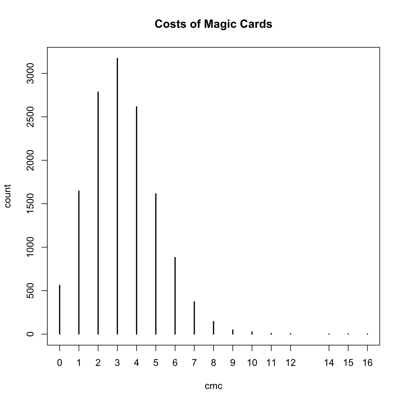
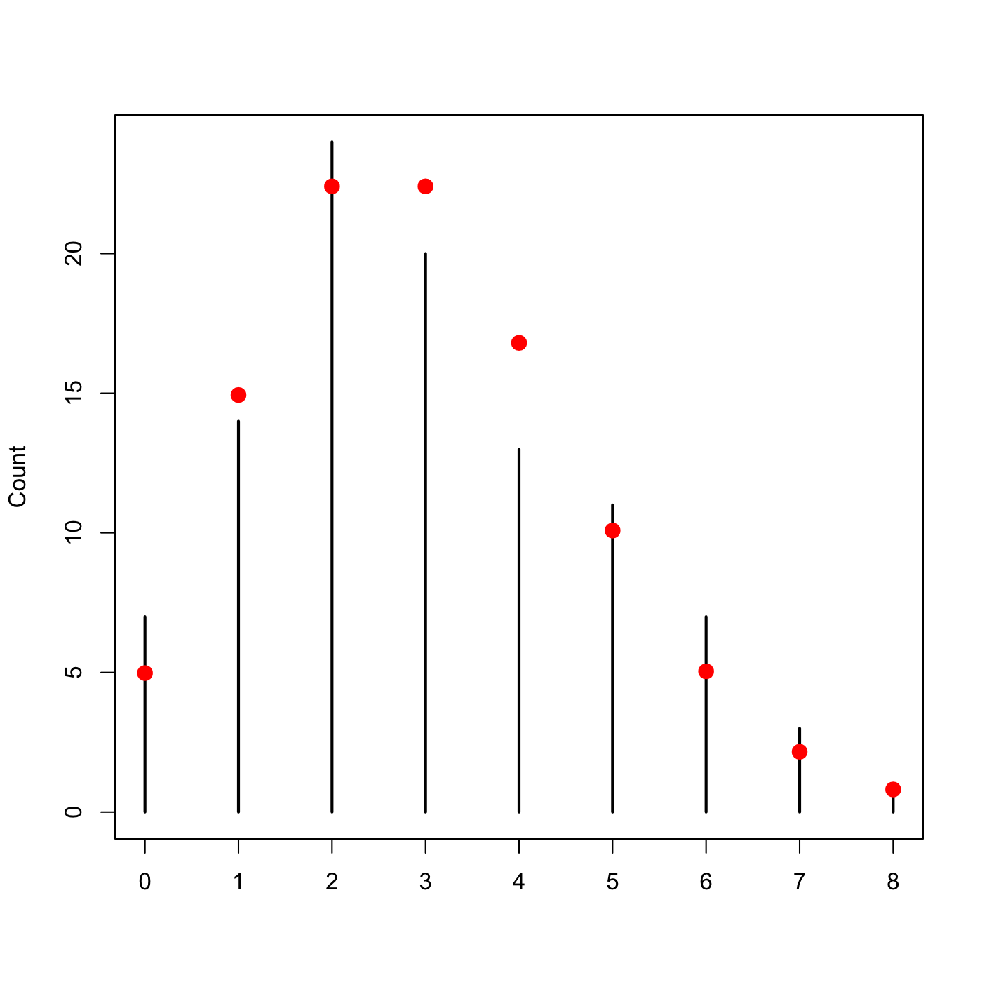
If you read Wednesday’s post where we recreated the London Blitz this should look very familiar. That’s right, the costs of Magic cards follow a Poisson distribution. We can add some points that show the appropriate Poisson distribution.

m <- mean(dat$cmc)
l <- length(dat$cmc)
comb <- 0:16
plot(table(dat$cmc),
	ylab='count',xlab='cmc',
	main='Costs of Magic Cards \n Poisson In Red')

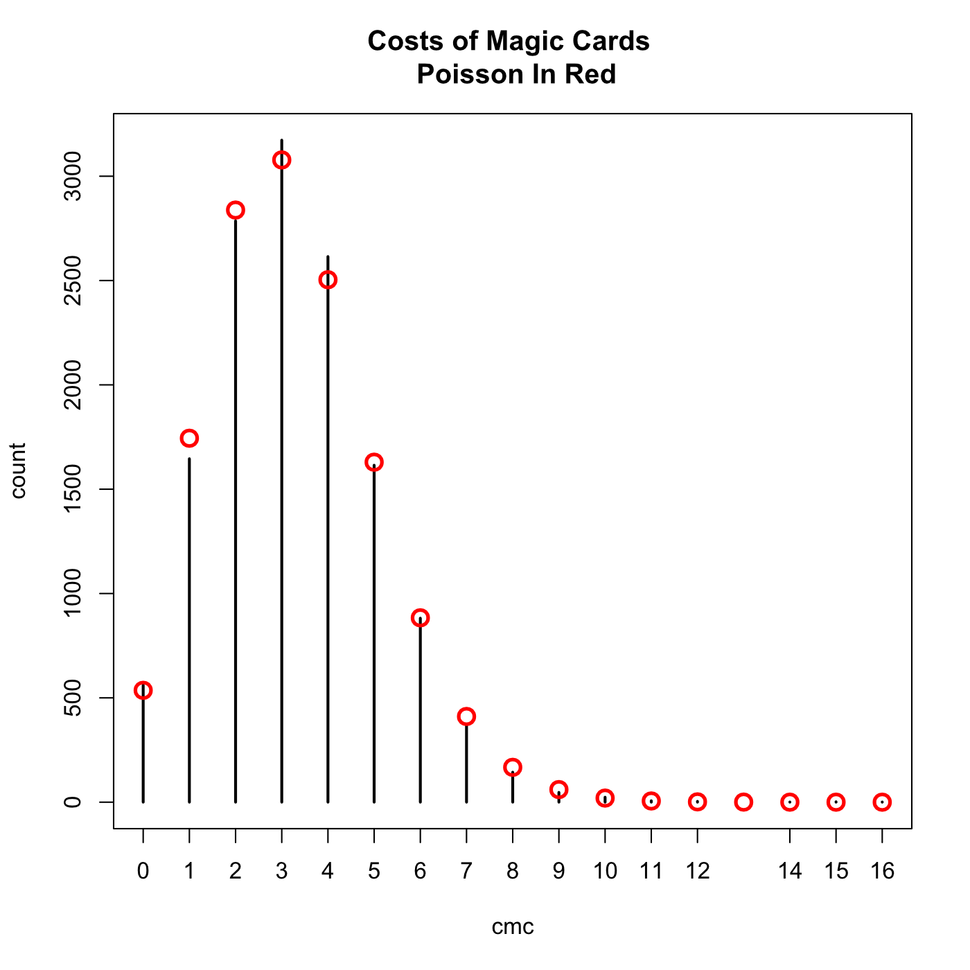
Its a ridiculously good fit, almost perfect. What is going on exactly? I mean I doubt they did this deliberately. When we last saw the Poisson distribution, and in almost every explanation of it you will ever find, the Poisson is the result of pure randomness. Are the design and development teams working blindfolded?

(Image from “Look At Me I’m The DCI” provided by mtgimage.com)
(Art by Mark Rosewater, Head Designer of Magic: The Gathering)

Nope. The secret is to think about where exactly the Poisson distribution comes from and forget its association with randomness. It requires that only zero and the natural numbers be valid possibilities and that a well defined average exists. Although Magic has never had a card which cost more than 16 mana there’s no actual limitation in place, high costs are just progressively less likely.

I expect that what we are seeing here is that the developers have found that keeping the mean cost of cards at around 3.25, in any given set, makes for good gameplay in the Limited format. Because they also want to keep their options open in terms of costs, a creature that costs more than 8 mana is a special occasion, the inevitable result is a Poisson distribution.

The Poission Distribution

The Poisson Distribution

The Poisson distribution is actually based on a relatively simple line of thought. How many times can an event occur in a certain period?

Let’s say that on an average day the help center gets 4 calls. Sometimes more and sometimes less. At any given moment we can either get a call or not get a call. This tells us that the probability distribution which describes how many calls we are likely to get each day is Binomial. Furthermore we know that it must be of the form Binomial(N,4/N) where where N is the greatest possible number of calls because this is the only way for the mean to be 4.

The question now becomes how many call is it possible to get in a day? Hard to say but presumably the phone could be ringing off the hook constantly. Its outrageously unlikely for me to get a hundred calls in a day but there is some probability that everyone in the building could need help on the same day. It is rarely possible to set an upper limit with confidence but watch what happens as we make the limit higher and higher.

As we increase the The distribution is converging on a particular shape. Poisson proved what the shape would become if N were infinite. He also showed that this new distribution was much easier to calculate the form of than the Binomial distribution. Since a very large N and an infinite N are nearly identical the difference is irrelevant so long as its possible for the event to happen a large number of times.

Since the Poisson distribution is effectively a Binomial distribution with N always set to the same value we can describe the Poisson using only the average rate. Here it is for an average rate of 4 events per interval (calls per day, meteor strikes per year, etc).

It is occasionally said the the Poisson distribution is the “law of rare events” which is a sort of true but mostly confusing title. What matters is that the event could potentially happen much more often than it does.

A switchboard that gets an average of 100 calls an hour is not getting calls “rarely” but it is going to follow a Poisson distribution because a call can happen at any moment during the hour. If the switchboard were very slow and could only handle one call every ten seconds (so never more than 360 calls in an hour) it would be better to use a binomial distribution.

When explaining things it is often better to show than tell. Let’s look at an example of how the Poisson arises.

The Blitz was a massive bombing of Britain during World War II. A major concern of the British government was whether or not the Nazi bombs were precise weapons. If the bombs were guided their policies to protect people in the cities would have to be different. The analysts knew that if the bombing were random the distribution of bombs would have to follow an approximately Poisson distribution.

We can simulate a bombing campaign pretty easily by creating a large number of random coordinates to represent for each hit. The city is ten kilometers by ten kilometers.

set.seed(10201)
x <- runif(300,0,10)
y <- runif(300,0,10)
xy <- data.frame(x,y)

And what does this attack look like? We’ll plot each point and overlay a 10×10 grid.

p <- ggplot(xy,aes(x=x,y=y))
p + geom_point(size=2.5,color='red') +
	geom_hline(yintercept=0:10) +
	geom_vline(xintercept=0:10) +
	scale_x_continuous(minor_breaks=NULL,breaks=NULL) +
	scale_y_continuous(minor_breaks=NULL,breaks=NULL) +
	coord_cartesian(xlim=c(0,10),ylim=c(0,10))

During the Blitz each square had to be counted up by hand. We can do a little better. The cut() function divides up the data into one hundred sections then we rename them into something easier to read.

xx <- cut(x,10)
yy <- cut(y,10)
levels(xx) <- 1:10
levels(yy) <- 1:10

A contingency table tells now tells us how many bombs landed in each square. As a dataframe its easier to work with. Making a plot to see how often each number of its came up is then very simple.

fr <- data.frame(table(xx,yy))
plot(table(fr$Freq))

It isn’t a perfect, fit, of course, but as we discussed about the philosophy of statistics we do not expect perfection. The trend is one that clearly approximates the Poisson distribution.